07 - DC and DR for each region per time (Figure 2)

07_V_scatterplot_Fig2.qmd

Note

The final figure presented in the manuscript is further edited with the aid of inkscape software

Domestic contribution (DC) and Domestic retention (DR) for all countries

Reading libraries

library(dplyr)    # Data manipulation
library(here)     # File path management
library(tidyr)    # Data tidying
library(ggplot2)  # Data visualization
library(scales)   # Scale transformations and labels
library(ggarrow)  # Adding arrows to ggplot

Here we combined two metrics, DC and DR by time and regions, to express the changes of NBTs distribution for each of these regions. This is aimed to be the Figure 02 in the manuscript. The Figure 2 in the main text was further edited in inkscape to better acomodate the arrows and include the quadrant information in the first plot.

# Data from 01_C_data_preparation.qmd

flow_period_region_prop <- readr::read_csv(here::here("data", "processed", "flow_period_region_prop.csv"))

Add lag values for visualization

flow_period_region_prop_lag <- flow_period_region_prop |>
  dplyr::group_by(region_type) |>
  dplyr::mutate(new_DC = dplyr::lag(prop_DC),
                new_DR = dplyr::lag(prop_DR)) |> 
  dplyr::ungroup()

Figure 2 - Scatterplot

flow_period_region_prop_lag |>
  dplyr::filter(dplyr::if_all(c(prop_DC, prop_DR, 
                                new_DC, new_DR), 
                              ~ . != 0 | is.na(.))) |> 
  ggplot(aes(x = prop_DC, y = prop_DR, fill = region_type))+
  geom_hline(yintercept = 0.5, linetype = "dashed")+
  geom_vline(xintercept = 0.5, linetype = "dashed")+
  geom_arrow_segment(
    aes(x = new_DC, xend = prop_DC,
        y = new_DR, yend = prop_DR),
    color = "grey",
    arrow_head = NULL,
    arrow_mid  = arrow_head_wings(offset = 30,
                                  inset = 60),
    resect_head = 2,
    resect_fins = 2
  )+
  geom_point(
    shape = 21,
    size = 2.5
  )+
  geom_point(
    aes(x = new_DC ,
        y = new_DR),
    alpha = 0.5,
    shape = 21,
    size = 2.5
  )+
  facet_wrap(.~period,axes = "all",
             axis.labels = "margins"
              )+
  scale_fill_manual(
    values = c(
      "Europe & Central Asia" = "#E64B35FF",
      "East Asia & Pacific" = "#4DBBD5FF",
      "North America" = "#3C5488FF",
      "South Asia" = "#B09C85FF",
      "Latin America & Caribbean" = "#00A087FF",
      "Sub-Saharan Africa" = "#F39B7FFF",
      "Middle East & North Africa" = "#8491B4FF"
    )
  )+
  scale_x_continuous(
    labels = scales::label_percent(),
    expand = expansion(mult = c(0.05, 0))
  )+
  scale_y_continuous(
    labels = scales::label_percent(),
    expand = expansion(mult = c(0.05, 0))
  )+
  labs(
    x = "Domestic Contribution (DC)",
    y = "Domestic Retention (DR)"
  )+
  theme_classic()+
  theme(
    strip.background = element_rect(fill = NA, color = NA),
    strip.text = element_text(face = "bold"),
    legend.position = "none",
    plot.background = element_blank(),
    panel.spacing = unit(5, "pt"),
    panel.spacing.x = unit(15, "pt"),
    plot.margin = margin(5,15,5,5,"pt"),
    axis.line = element_line(lineend = "round"),
    axis.text = element_text(color = "black"),
    axis.ticks = element_line(color = "black")
  )+
  coord_cartesian(xlim = c(0,1),
                  ylim = c(0,1),
                  clip = "off")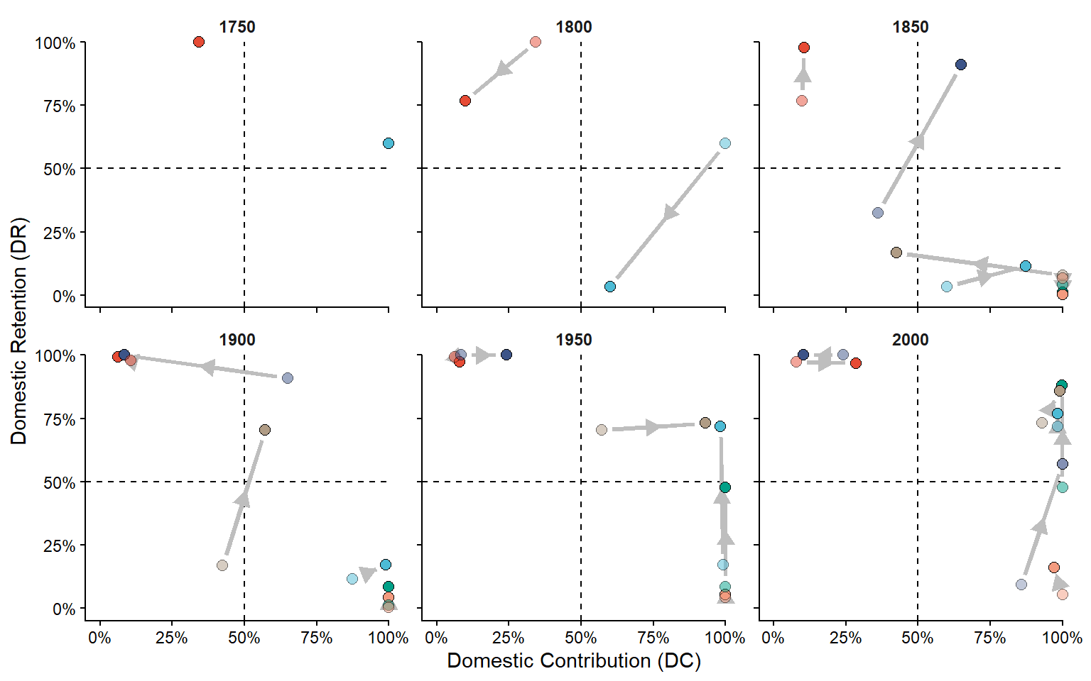

ggsave(filename = here::here("output", "figures", "Fig2_DC_DR.png"), 
       width = 8, height = 5)