04 - Modelling different aspects of countries regarding name bearers characteristics

04_A_model_NBTs.qmd

General overview

Here we provided the code used to model the total number of name bearers, endemic deficit and non-endemic representation. These models are represented in Figures 3 in the main text, Figure S2 and S3, and tables S1, S2 and S3 in Supplementary material.

Reading libraries

# data
library(dplyr)       # data manipulation
library(readr)       # read CSV files
library(here)        # file paths handling

# plot
library(scales)      # data transformation functions
library(ggplot2)     # data visualization

# model
library(glmmTMB)     # generalized Linear Mixed Models
library(performance) # model performance checks
library(bbmle)       # model selection and AIC calculations
library(DHARMa)      # model diagnostics and residuals simulation

Previous data used

# Data from 02_C_data_preparation_models.qmd
df_country_complete6 <- readr::read_csv(here::here("data", "processed", "df_country_complete6.csv"))

Some auxiliary function used to plot the results

sqrt_trans <- scales::trans_new("sqrt_with_zero", 
                        transform = function(x) ifelse(x == 0, 0, sqrt(x)),
                        inverse = function(x) x^2)

Modelling primary type distribution with biological and sociological/economic/political variables

In the modelling approach we used four response variables:

The total number of name bearers owned by a country total_country_museum
The rate of endemic deficit by a country native.beta
The rate of non-endemic representation by a country type.beta

All these variables are used in a country level (i.e. each point in the figures corresponds to a country)

Data and Models

Total number of name bearers by country

After standardize the variables we can fit the models. Since we have a huge amount of zeroes in our response variable we will use a zero-inflation poisson model and also test with a poisson distribution.

ggplot(df_country_complete6, aes(type.richness.pad)) +
  geom_density(alpha = 0.4, fill = "darkorange")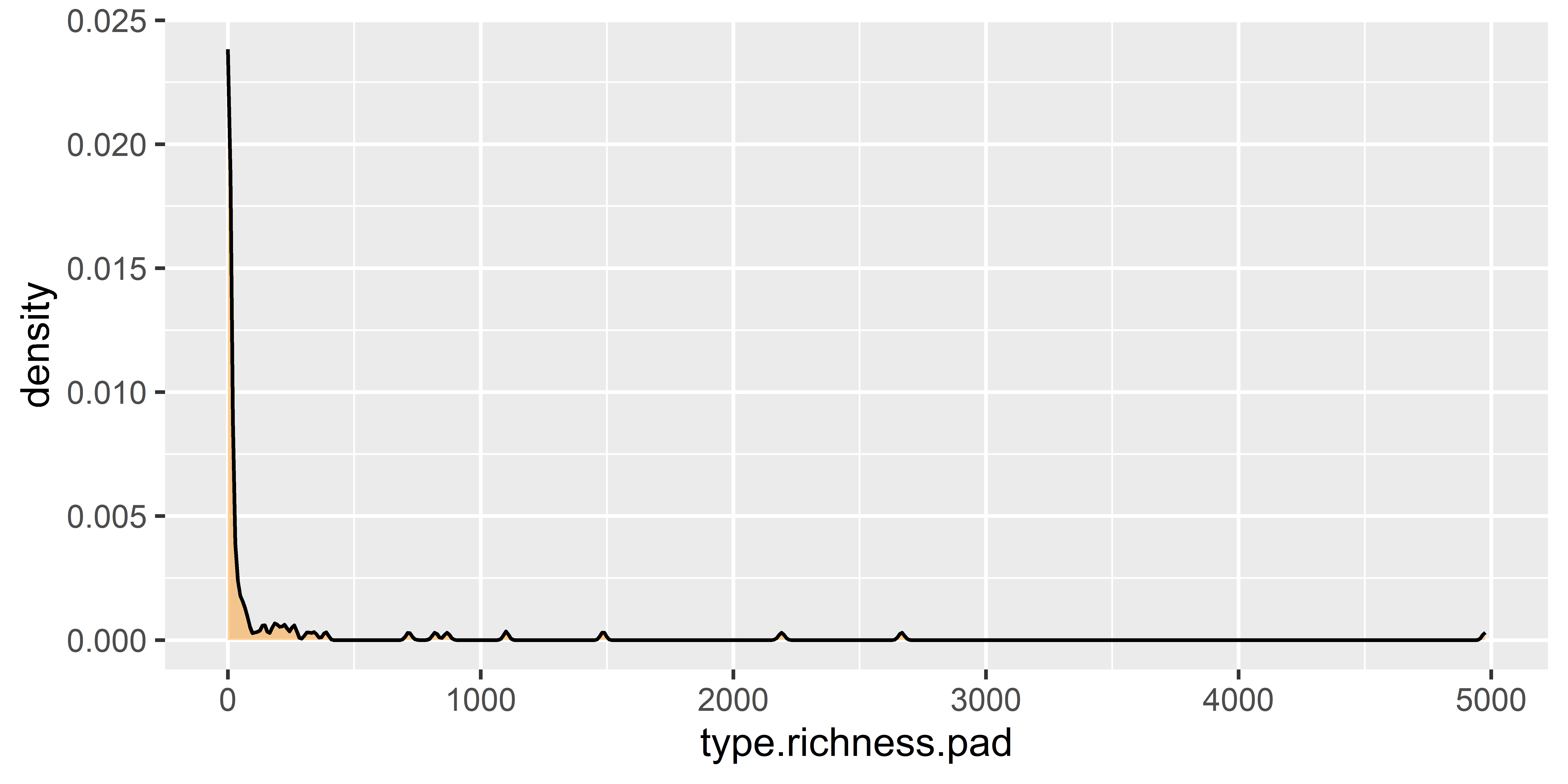

Fitting different models to check which one is the most appropriate

mod_pois <-
  glmmTMB::glmmTMB(type.richness.pad ~ native.richness.pad + 
                     records.per.area.pad + years.independence.pad + 
                     gdp.pad + n.museums.pad, zi = ~., 
                   data = df_country_complete6, 
                   family = poisson) # poisson

mod_zero_pois <-
  glmmTMB::glmmTMB(type.richness.pad ~ native.richness.pad + 
                     records.per.area.pad + years.independence.pad + 
                     gdp.pad + n.museums.pad, zi = ~., 
                   data = df_country_complete6, 
                   family = glmmTMB::nbinom2) # negative binomial

mod_hurdle <-
  glmmTMB::glmmTMB(type.richness.pad ~ native.richness.pad +
                     records.per.area.pad + years.independence.pad +
                     gdp.pad + n.museums.pad,
                   zi = ~.,
                   data = df_country_complete6,
                   family = glmmTMB::truncated_nbinom2)

Checking model output and fit

summary(mod_hurdle)
performance::check_zeroinflation(mod_hurdle)
summary(mod_zero_pois)
performance::check_zeroinflation(mod_zero_pois)

Checking best model

## model selection
bbmle::ICtab(mod_pois, mod_zero_pois, mod_hurdle)

Checking residual diagnostic and colinearity

# checking homocedasticity 
DHARMa::simulateResiduals(fittedModel = mod_zero_pois, plot = T)
DHARMa::simulateResiduals(fittedModel = mod_hurdle, plot = T)
performance::check_collinearity(mod_zero_pois)
performance::check_collinearity(mod_hurdle)

Exporting best model

# Exporting best model

saveRDS(mod_zero_pois, here::here("output", "models", "model_res_counting.rds"))

Modelling endemic deficit and non-endemic representation

In this section we will model endemic deficit and non-endemic representation. These variables are under the names native.beta and type.beta.

mod_native_turnover <-
  glmmTMB::glmmTMB(cbind(native.success, native.fail) ~ native.richness.pad +
                     records.per.area.pad + years.independence.pad +
                     gdp.pad + n.museums.pad, 
                   family = glmmTMB::betabinomial,
                   data = df_country_complete6)


mod_type_turnover <-
  glmmTMB::glmmTMB(cbind(type.success, type.fail) ~ native.richness.pad +
                     records.per.area.pad + years.independence.pad +
                     gdp.pad + n.museums.pad, 
                   family = glmmTMB::betabinomial,
                   data = df_country_complete6)

Checking model outputs

## Diagnose plots
summary(mod_native_turnover)
summary(mod_type_turnover)

Checking residuals and colinearity

DHARMa::simulateResiduals(fittedModel = mod_native_turnover, plot = TRUE)
DHARMa::simulateResiduals(fittedModel = mod_type_turnover, plot = TRUE)
performance::check_collinearity(mod_native_turnover)
performance::check_collinearity(mod_type_turnover)

Saving models

# Saving models

saveRDS(mod_native_turnover, here::here("output", "models", "model_res_turnover_native.rds"))
saveRDS(mod_type_turnover, here::here("output", "models", "model_res_turnover_nbt.rds"))