library(circlize)  #chord diagrams
library(dplyr)     #data manipulation
library(glue) #string interpolation05 - Producing chord diagram (Figure 1)
05_V_chord_diagram_Fig1.qmd
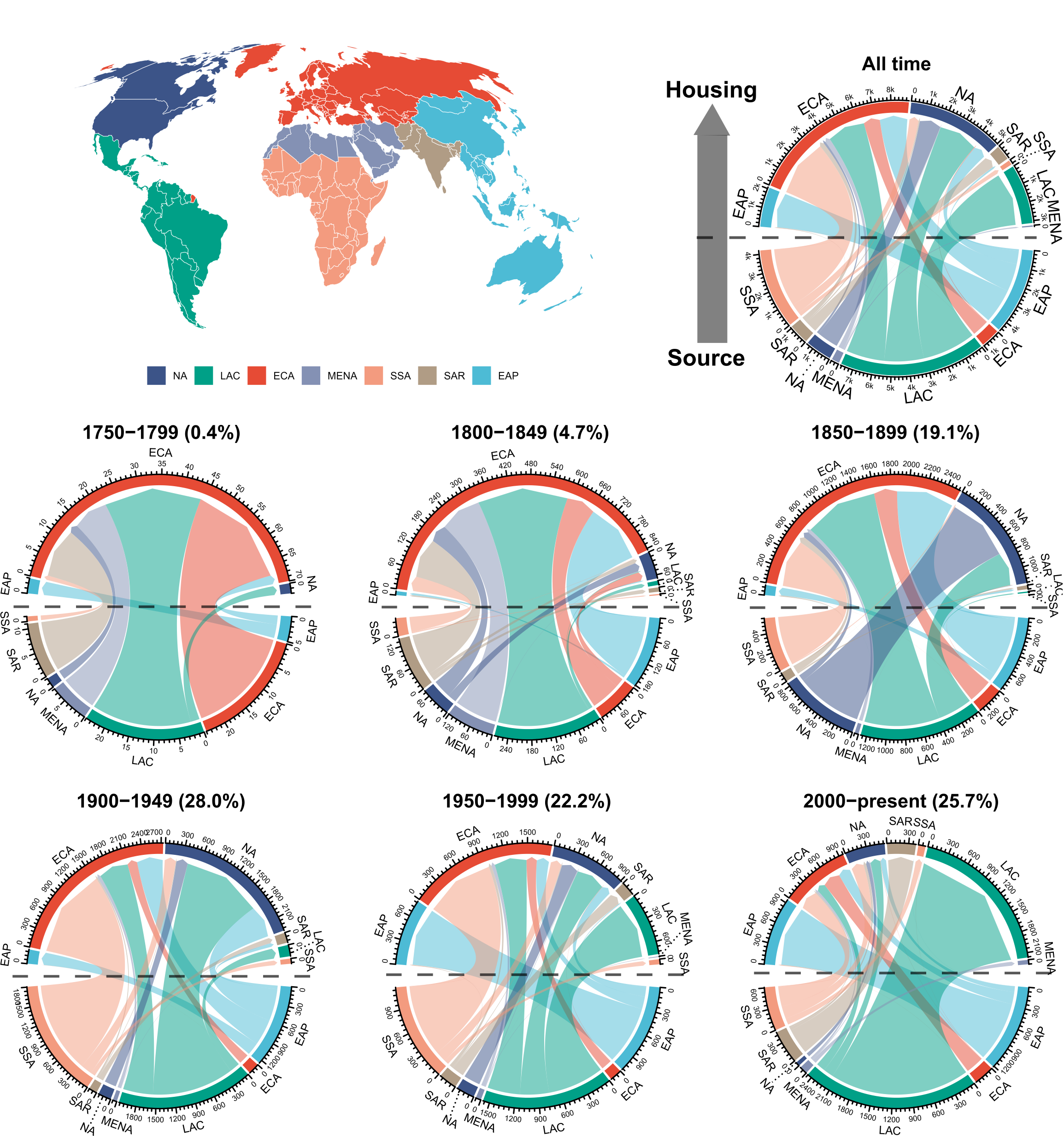
Here we produce the chord diagram (Figure 1 in the manuscript)
Data used in this script
# Data from 01_C_data_preparation.qmd
flow_period_region <- readr::read_csv(here::here("data", "processed", "flow_period_region.csv"))

flow_region <- readr::read_csv(here::here("data", "processed", "flow_region.csv"))
Mapping name bearers flow among regions per time interval of 50 years
# use region abbreviation
flow_period_region2 <- flow_period_region |>
  dplyr::mutate(
    dplyr::across(
      c(region_type, region_museum),
      ~dplyr::case_when(
        . == "Europe & Central Asia" ~ "ECA",
        . == "East Asia & Pacific" ~ "EAP",
        . == "North America" ~ "NA",
        . == "South Asia" ~ "SAR",
        . == "Latin America & Caribbean" ~ "LAC",
        . == "Sub-Saharan Africa" ~ "SSA",
        . == "Middle East & North Africa" ~ "MENA"
      )))

flow_region2 <- flow_region |>
  dplyr::mutate(
    dplyr::across(
      c(region_type, region_museum),
      ~dplyr::case_when(
        . == "Europe & Central Asia" ~ "ECA",
        . == "East Asia & Pacific" ~ "EAP",
        . == "North America" ~ "NA",
        . == "South Asia" ~ "SAR",
        . == "Latin America & Caribbean" ~ "LAC",
        . == "Sub-Saharan Africa" ~ "SSA",
        . == "Middle East & North Africa" ~ "MENA"
      )))

# create dataset for each region

regions_1750 <- flow_period_region2 |>
  dplyr::filter(period == 1750) |>
  dplyr::select(-c(period, total_period_region_type)) |>
  dplyr::mutate(
    region_type = glue::glue(" {region_type}"),
    region_museum = glue::glue("{region_museum} ")) |>
  dplyr::rename(
    from = region_type,
    to = region_museum,
    value = n) |>
  dplyr::filter(
    value != 0
  )

regions_1800 <- flow_period_region2 |>
  dplyr::filter(period == 1800) |>
  dplyr::select(-c(period, total_period_region_type)) |>
  dplyr::mutate(
    region_type = glue::glue(" {region_type}"),
    region_museum = glue::glue("{region_museum} ")) |>
  dplyr::rename(
    from = region_type,
    to = region_museum,
    value = n) |>
  dplyr::filter(
    value != 0
  )

regions_1850 <- flow_period_region2 |>
  dplyr::filter(period == 1850) |>
  dplyr::select(-c(period, total_period_region_type)) |>
  dplyr::mutate(
    region_type = glue::glue(" {region_type}"),
    region_museum = glue::glue("{region_museum} ")) |>
  dplyr::rename(
    from = region_type,
    to = region_museum,
    value = n) |>
  dplyr::filter(
    value != 0
  )

regions_1900 <- flow_period_region2 |>
  dplyr::filter(period == 1900) |>
  dplyr::select(-c(period, total_period_region_type)) |>
  dplyr::mutate(
    region_type = glue::glue(" {region_type}"),
    region_museum = glue::glue("{region_museum} ")) |>
  dplyr::rename(
    from = region_type,
    to = region_museum,
    value = n) |>
  dplyr::filter(
    value != 0
  )

regions_1950 <- flow_period_region2 |>
  dplyr::filter(period == 1950) |>
  dplyr::select(-c(period, total_period_region_type)) |>
  dplyr::mutate(
    region_type = glue::glue(" {region_type}"),
    region_museum = glue::glue("{region_museum} ")) |>
  dplyr::rename(
    from = region_type,
    to = region_museum,
    value = n) |>
  dplyr::filter(
    value != 0
  )

regions_2000 <- flow_period_region2 |>
  dplyr::filter(period == 2000) |>
  dplyr::select(-c(period, total_period_region_type)) |>
  dplyr::mutate(
    region_type = glue::glue(" {region_type}"),
    region_museum = glue::glue("{region_museum} ")) |>
  dplyr::rename(
    from = region_type,
    to = region_museum,
    value = n) |>
  dplyr::filter(value != 0)

regions_alltime <- flow_region2 |>
  dplyr::select(-total_region_type) |>
  dplyr::mutate(
    region_type = glue::glue(" {region_type}"),
    region_museum = glue::glue("{region_museum} ")) |>
  dplyr::rename(
    from = region_type,
    to = region_museum,
    value = n) |>
  dplyr::filter(value != 0)

#define colors
colors <- c(
  " ECA" = "#f34d4d",
  " EAP" = "#4da8a6",
  " NA" = "#416295",
  " SAR" = "#a6a7a6",
  " LAC" = "#4dae7d",
  " SSA" = "#E0A0A7",
  " MENA" = "#9D7AAB",
  "ECA " = "#f34d4d",
  "EAP " = "#4da8a6",
  "NA " = "#416295",
  "SAR " = "#a6a7a6",
  "LAC " = "#4dae7d",
  "SSA " = "#E0A0A7",
  "MENA " = "#9D7AAB"
)
Producing the figures
#start pdf
pdf(here::here("output", "figures", "Fig1.pdf"), width = 8, height = 8)

#define layout
# The layout will follow this order
# 1 4 7
# 2 5 8
# 3 6 9
layout(matrix(1:9, 3, 3))

#1 - blank space for map
plot(0, type='n', axes=FALSE, ann=FALSE)

#2 - 1750-1799
chordDiagram(regions_1750,
             grid.col = colors,
             directional = 1,
             direction.type = c("arrows"),
             link.arr.type = "big.arrow",
             reduce = 0.000000000000001,
)
title("1750-1799")

#3 - 1900-1949
chordDiagram(regions_1900,
             grid.col = colors,
             directional = 1,
             direction.type = c("arrows"),
             link.arr.type = "big.arrow",
             reduce = 0.000000000000001,
)
title("1900-1949")

#4 - blank space for map
plot(0, type='n', axes=FALSE, ann=FALSE)

#5 - 1800-1849
chordDiagram(regions_1800,
             grid.col = colors,
             directional = 1,
             direction.type = c("arrows"),
             link.arr.type = "big.arrow",
             reduce = 0.000000000000001,
)
title("1800-1849")

#6 - 1950-1999
chordDiagram(regions_1950,
             grid.col = colors,
             directional = 1,
             direction.type = c("arrows"),
             link.arr.type = "big.arrow",
             reduce = 0.000000000000001,
)
title("1950-1999")

#7 - All time
chordDiagram(regions_alltime,
             grid.col = colors,
             directional = 1,
             direction.type = c("arrows"),
             link.arr.type = "big.arrow",
             annotationTrack = "grid",
             reduce = 0.000000000000001,
             preAllocateTracks = list(track.height = 0.1,
                                      track.margin = c(0,0)),
             annotationTrackHeight = mm_h(c(2, 2)),
             )

circos.track(track.index = 1, panel.fun = function(x, y) {
  if(abs(CELL_META$cell.start.degree - CELL_META$cell.end.degree) > 0) {
    sn = CELL_META$sector.index
    i_state = as.numeric(gsub("(C|R)_", "", sn))
    circos.text(CELL_META$xcenter, 1, CELL_META$sector.index,
                facing = "inside", niceFacing = TRUE, adj = c(0.5,0))
    xlim = CELL_META$xlim
    breaks = seq(0, 10000, by = 1000)
    circos.axis(
      major.at = breaks,
      labels = ifelse(breaks >= 1000, paste0(breaks/1000, "k"), breaks),
      labels.cex = 0.5,
      h = "bottom"
      )
  }
}, bg.border = NA)

title("All time")

#8 - 1850-1899
chordDiagram(regions_1850,
             grid.col = colors,
             directional = 1,
             direction.type = c("arrows"),
             link.arr.type = "big.arrow",
             reduce = 0.000000000000001,
)
title("1850-1899")

#9 - 2000-present
chordDiagram(regions_2000,
             grid.col = colors,
             directional = 1,
             direction.type = c("arrows"),
             link.arr.type = "big.arrow",
             reduce = 0.000000000000001,
)
title("2000-present")

#Finish
dev.off()
png
2 circos.clear()Plotting the final figure
Note
The manuscript version of this Figure is edited with Inkscape software
This is the final figure that correspond to the Figure 1 of the manuscript