library(readr) # read csv objects
library(dplyr) # manipulate tables
library(tidyr) # data tidying
library(ggplot2) # plot figures
library(scales) # change axis values
library(countrycode) # download country informationSupplementary material - Figures and Tables
0010_Supplementary_analysis.qmd
In this document we provide the code to reproduce the Figures and Tables presented in supplementary material of the manuscript “The macroecology of knowledge: Spatio-temporal patterns of name-bearing types in biodiversity science”
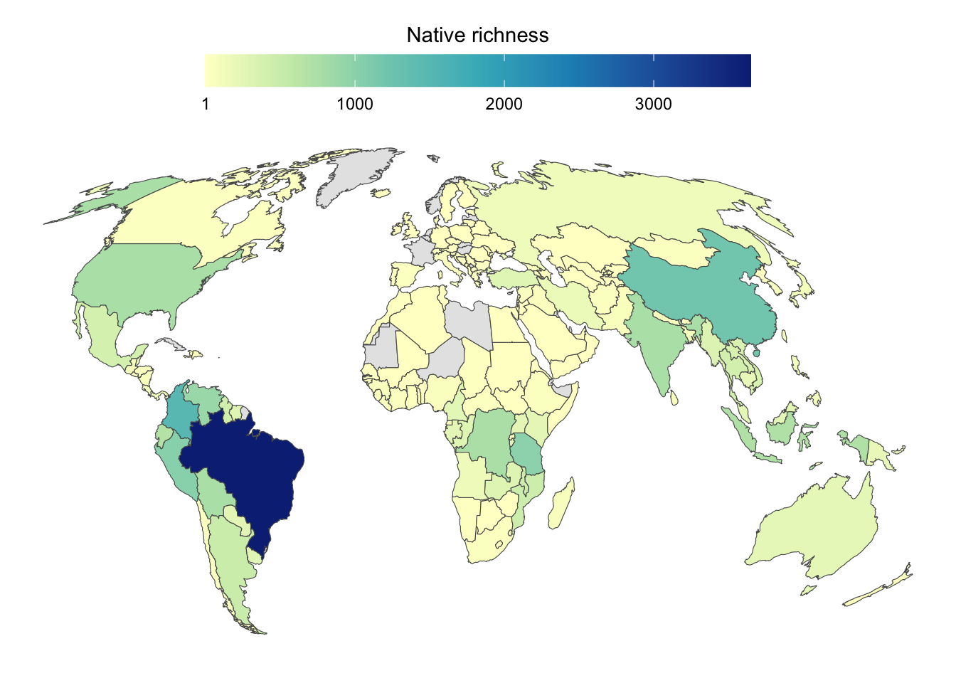
Native species richness
Native richness with Catalog of Fishes
We calculate the native species richness for each country from data in the Catalog of Fishes. We used this source to avoid taxonomic mismatches between species names.
# Data from 01_C_data_preparation.qmd
df_country_native <- readr::read_csv(file = here::here("data","processed", "df_country_native.csv"))
countries <-
rnaturalearth::ne_countries(scale = "medium",
returnclass = "sf") |>
dplyr::filter(region_wb != "Antarctica")|>
rmapshaper::ms_filter_islands(min_area = 20000000000) |>
rmapshaper::ms_simplify(keep = 0.95)
sf_countries <-
sf::st_as_sf(countries) |>
dplyr::filter(admin != "Antarctica") |>
dplyr::select(iso_a3)
df_country_native_sf <-
sf_countries |>
dplyr::full_join(df_country_native,
by = c(iso_a3 = "country_distribution"))Comparing richness from the Catalog of Fishes and Fishbase
Here we compared the richness obtained from the Catalog of Fishes and the Fishbase.
df_country_native_fishbase <- readr::read_csv(file = here::here("data","processed", "fishbase_species_country.csv"))

df_country_native_fishbase2 <-
  df_country_native_fishbase |>
  dplyr::rename(iso3c.fishbase = iso3c)

df_richness_all <-
  df_country_native |>
  dplyr::left_join(df_country_native_fishbase2, by = c(country_distribution = "iso3c.fishbase")) |>
  tidyr::drop_na()

cor(df_richness_all$native.richness, df_richness_all$n)
[1] 0.898011Figure S1 - Native richness
Native richness was extracted from the Catalog of Fishes
df_country_native_sf |>
  ggplot()+
  geom_sf(aes(fill = native.richness))+
  scale_fill_distiller(palette = "YlGnBu",
                       direction = 1,
                       na.value = "grey90",
                       breaks = c(1, 1000, 2000,3000, 3854))+
  labs(
    fill = "Native richness"
  )+
  guides(fill = guide_colorbar(barwidth = 20))+
  theme_void()+
  theme(
    legend.position = "top",
    legend.title.position = "top",
    legend.title = element_text(hjust = 0.5),
    plot.background = element_rect(fill = "white",
                                   color = NA)
  )+
  coord_sf(
    crs = "+proj=moll +x_50=0 +y_0=0 +lat_0=0 +lon_0=0"
    )
ggsave(here::here("output", "figures",
                  "Supp-material", "FigS1_native_richness.png"),
       width = 7, height = 5, dpi = 600)
Calculating native deficit and non-native representation metrics with full native dataset
Reading packages
# data
library(readr)        # reading CSV files
library(here)         # constructing file paths
library(dplyr)        # data manipulation
library(tidyr)        # data tidying
library(phyloregion)  # handling phylogenetic data and transformations
Importing and processing data
Importing and processing native composition and name bearer composition data
# From 01_C_data_preparation.qmd
spp_native_distribution <- readr::read_csv(here::here("data", "raw", "spp_native_distribution.csv"))

# From 01_C_data_preparation.qmd
spp_type_distribution <- readr::read_csv(here::here("data", "raw", "spp_type_distribution.csv"))
Checking the specimens with data in both tables (native distribution and types). We transformed the long format species occurrence data frame to dense format. During this procedure we removed 1204 species that do not have information on native distribution (or we couldn’t get this information from CAS)
df_native_grid <-
  spp_native_distribution |>
  dplyr::select(grids = country_distribution,
                species = species) |>
  tidyr::drop_na(grids)

df_type_grid <-
  spp_type_distribution |>
  dplyr::select(grids = country_museum,
                species = species) |>
  tidyr::drop_na(grids) |>
  dplyr::mutate(grids = paste(grids, "type", sep = "_"))


# joining data frames
df_all_grid <- rbind(df_native_grid, df_type_grid) # joining both matrices -
    #native and types composition

#### Just descriptive quantities
country_native <- unique(df_native_grid$grids)
country_type <- gsub(pattern = "_type",
                     replacement = "",
                     unique(df_type_grid$grids))
country_type_zero <- setdiff(country_native, country_type) # countries with no type specimen

# transforming into a sparse matrix to speed up calculations
sparse_all <- df_all_grid |>
  phyloregion::long2sparse(grids = "grids", species = "species") |>
  phyloregion::sparse2dense()

# Transforming in presence absence matrix
sparse_all_pa <- ifelse(sparse_all >= 1, 1, 0)

# Binding countries with no types - adding zeroes
country_type_zero_names <- paste(country_type_zero, "_type", sep = "") # this will be used to bind together matrix with types and add the countries with no type
matrix_type_zero <- matrix(0,
         nrow = length(country_type_zero_names),
         ncol = ncol(sparse_all_pa),
         dimnames = list(country_type_zero_names,
                         colnames(sparse_all_pa)))

sparse_all_pa2 <- rbind(sparse_all_pa, matrix_type_zero)
Calculating native defict and non-native representation
Here we calculate the values of native deficit (proportion of native species lacking in a country’s biological collections) and the proportion of name bearers that corresponds to non native species
source(here::here("R", "functions", "function_beta_types_success_fail.R"))

names_countries <- unique(df_native_grid$grids) # country names

df_all_beta <- beta_types(presab = sparse_all_pa2,
                          names.countries = names_countries) # calculating metrics of directional turnover

readr::write_csv(df_all_beta, here::here("data", "processed", "df_all_beta.csv"))
Plotting native deficit and non-native representation for each country
In this section we present the cartogram of world map with values of native deficit and non-native representation using the full dataset of native species (Figure S2)
Loading packages
#data
library(dplyr)
library(tidyr)
#plot
library(ggplot2)
library(patchwork)
library(cowplot)
#map
library(rnaturalearth)
library(rmapshaper)
library(sf)
library(biscale)
Data
# Data from 02_D_beta-countries.qmd
df_all_beta <- readr::read_csv(here::here("data", "processed", "df_all_beta.csv"))
Joining metric information with geographical data
countries <- rnaturalearth::ne_countries(returnclass = "sf")

sf_countries <-
  sf::st_as_sf(countries) |>
  dplyr::filter(admin != "Antarctica") |>
  sf::st_transform(crs = "+proj=moll +x_0=0 +y_0=0 +lat_0=0 +lon_0=0") |>
  dplyr::select(iso_a3_eh)

df_all_beta_sf <-
  sf_countries |>
  dplyr::full_join(df_all_beta, by = c(iso_a3_eh = "countries"))
First processing spatial data to convert NA values into 0
df_all_beta_sf2 <-
  df_all_beta_sf |>
  sf::st_as_sf() |>
  rmapshaper::ms_filter_islands(min_area = 12391399903) |>
  dplyr::mutate(
    type.beta = ifelse(is.na(type.beta),
                           0,
                           type.beta),
    native.beta = ifelse(is.na(native.beta),
                           0,
                           native.beta))
Create palettes
palette_blue <- colorRampPalette(c("#d3d3d3", "#accaca", "#81c1c1", "#52b6b6"))

palette_pink <- colorRampPalette(c("#d3d3d3", "#c5acc2", "#bb84b1", "#ac5a9c"))
Plotting maps
map_native_beta <-
  ggplot() +
  geom_sf(data = df_all_beta_sf2,
          aes(geometry = geometry,
              fill = native.beta),
          color = "white",
          size = 0.1, na.rm = T) +
  scale_fill_gradientn(
    colors = palette_pink(10),
    na.value = "#d3d3d3",
    limits = c(0,1)
  )+
  guides(fill = guide_colorbar(
    barheight = unit(0.1, units = "in"),
    barwidth =  unit(4, units = "in"),
    ticks.colour = "grey20",
    title.position="top",
    title.hjust = 0.5
  )) +
  labs(
    fill = "Native deficit"
  )+
  theme_classic()+
  theme(
    legend.position = "bottom",
    legend.margin = margin(-10,0,0,0,"pt"),
    axis.text = element_blank(),
    axis.ticks = element_blank(),
    axis.line = element_blank()
  )

map_type_beta <-
  ggplot() +
  geom_sf(data = df_all_beta_sf2,
          aes(geometry = geometry,
              fill = type.beta),
          color = "white",
          size = 0.1, na.rm = T) +
  scale_fill_gradientn(
    colors = palette_blue(10),
    na.value = "#d3d3d3",
    limits = c(0,1)
  )+
  guides(fill = guide_colorbar(
    barheight = unit(0.1, units = "in"),
    barwidth =  unit(4, units = "in"),
    ticks.colour = "grey20",
    title.position="top",
    title.hjust = 0.5
  )) +
  labs(
    fill = "Non-native representation"
  )+
  theme_classic()+
  theme(
    legend.position = "bottom",
    legend.margin = margin(-10,0,0,0,"pt"),
    axis.text = element_blank(),
    axis.ticks = element_blank(),
    axis.line = element_blank()
  )
Plotting the two quantities in a bivariate map
sf_bivar_types <-
  bi_class(df_all_beta_sf2,
           x = type.beta,
           y = native.beta,
           style = "equal",
           dim = 4)

bivar_map_types <-
  ggplot() +
  geom_sf(data = sf_bivar_types,
          aes(geometry = geometry,
              fill = bi_class),
          color = "white",
          size = 0.1,
          show.legend = FALSE) +
  bi_scale_fill(pal = "DkBlue2",
                dim = 4) +
  theme_classic()+
  theme(
    legend.position = "bottom",
    legend.title = element_blank(),
        axis.text = element_blank(),
        axis.ticks = element_blank(),
        axis.line = element_blank(),
    panel.background = element_rect(fill = NA),
    plot.background = element_rect(fill = NA)
  )

legend <-
  bi_legend(pal = "DkBlue2",
            dim = 4,
            xlab = "Non-native",
            ylab = "Native deficit",
            size = )

bivar_map_type_final <-
  ggdraw() +
  draw_plot(legend, 0.0, 0.15, 0.25, 0.25) +
  draw_plot(bivar_map_types, 0, 0, 1, 1)
Joining all the maps
map_turnover_all <-
  map_native_beta+map_type_beta+bivar_map_type_final+
  patchwork::plot_layout(
    design =
"AB
 CC"
  )+
  patchwork::plot_annotation(tag_levels = "a")&
  theme(
    plot.tag = element_text(face = "bold", hjust = 0, vjust = 1),
    plot.tag.position = c(0, 1),
  )
map_turnover_all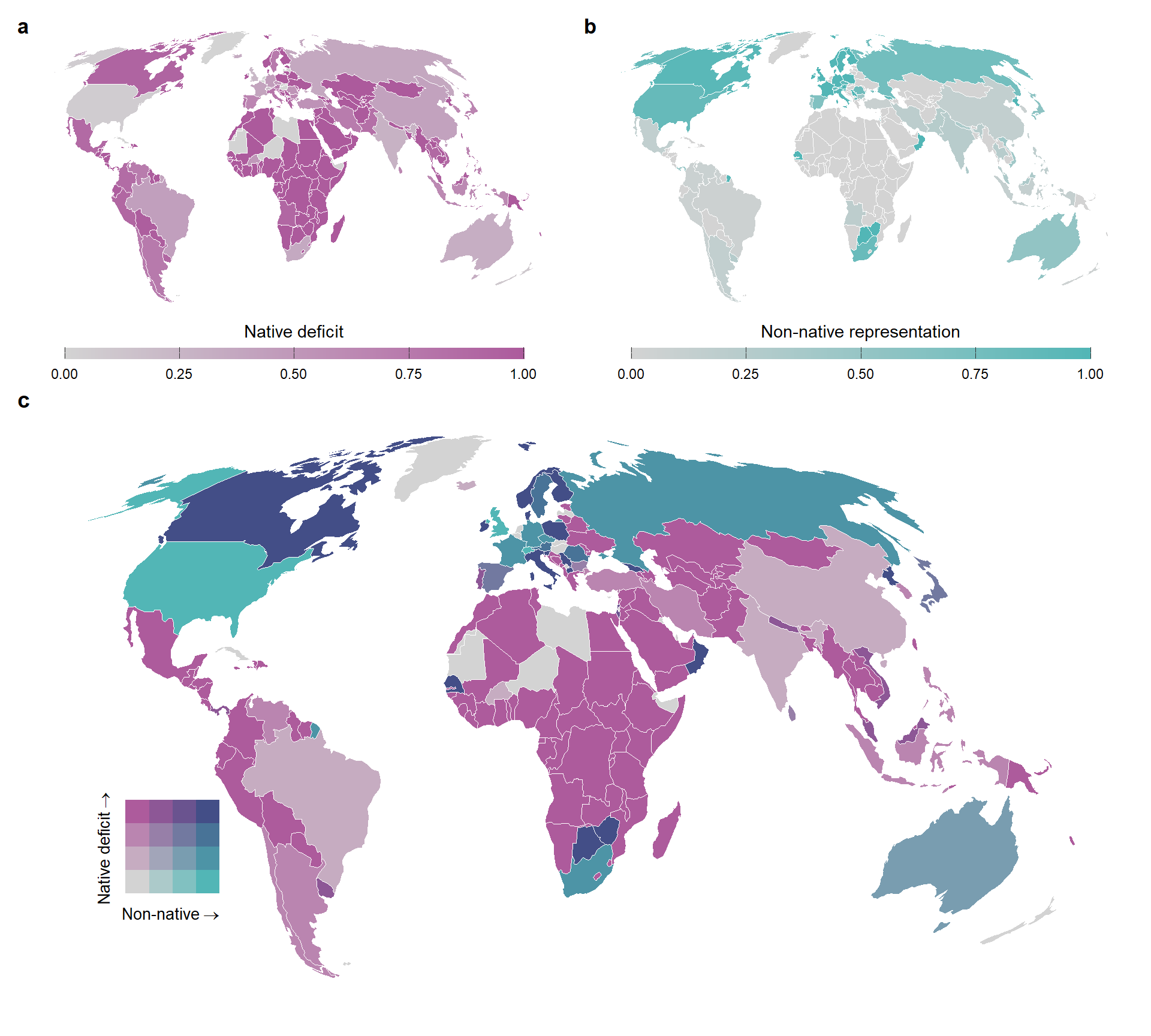
ggsave(here::here("output", "figures", "Supp-material", "FigS3_turnover_metrics.png"),
       map_turnover_all, dpi=600, width = 10, height = 9)
Comparison between full dataset and endemic dataset
We performed correlations between native deficit and non-native representation calculated using the endemic dataset and the full dataset of native species
df_endemic_beta <- readr::read_csv(here::here("data", "processed", "df_endemic_beta.csv"))

df_endemic_beta2 <-
  df_endemic_beta |>
  tidyr::drop_na(type.beta)
df_all_beta_sf2 <-
  df_all_beta_sf |>
  tidyr::drop_na(type.beta)

df_cor <-
  df_endemic_beta2 |>
  dplyr::left_join(df_all_beta_sf2, by = c(countries = "iso_a3_eh"))

cor(df_cor$type.beta.x, df_cor$type.beta.y)
[1] 0.8185594cor(df_cor$native.beta.x, df_cor$native.beta.y)[1] 0.893118Model results
Here we report tables containing full results of the generalized linear models presented in the main text . Also we report residuals diagnostic plots using DHARMa package
library(sjPlot)    # creating summary tables of model results
library(glmmTMB)   # read model output objects
library(DHARMa)    # diagnostic graphics of models
library(here)      # constructing file paths
Model data
Reading model results
# Data from 03_C_data_preparation.qmd
df_country_complete6 <- readr::read_csv(here::here("data", "processed", "df_country_complete6.csv"))

# Data from 04_D_model_NBTs.qmd
mod_counting_NBT <- readRDS(here::here("output",
                                       "models",
                                       "model_res_counting.rds")) # NBT total countings
mod_turnover_native <- readRDS(here::here("output",
                                          "models",
                                      "model_res_turnover_native.rds"))
mod_turnover_nbt <- readRDS(here::here("output",
                                       "models",
                                       "model_res_turnover_nbt.rds"))
Tables with estimated parameters
Producing tables with model parameters. These tables corresponds to the Tables S1 to S5 in the Supplementary material
# Table with model parameters for total number of NBT
sjPlot::tab_model(mod_counting_NBT,
                  transform = NULL,
                  pred.labels = c("Intercept",
                                  "Native richness",
                                  "Gbif records per area",
                                  "Years since independence",
                                  "GDP",
                                  "Number of museums",
                                  "Dispersion parameter"),
                  dv.labels = "Total Name Bearing Types",
                  string.pred = "Coefficients",
                  string.est = "Estimates",
string.p = "P-value")| Total Name Bearing Types | ||||
| Coefficients | Estimates | CI | P-value | |
| Count Model | ||||
| Intercept | 3.64 | 3.20 – 4.09 | <0.001 | |
| Native richness | 0.67 | 0.07 – 1.28 | 0.030 | |
| Gbif records per area | 0.36 | -0.00 – 0.73 | 0.052 | |
| Years since independence | -0.03 | -0.41 – 0.35 | 0.879 | |
| GDP | 0.84 | 0.37 – 1.31 | <0.001 | |
| Number of museums | 0.62 | 0.13 – 1.10 | 0.013 | |
| Dispersion parameter | 0.46 | 0.33 – 0.65 | ||
| Zero-Inflated Model | ||||
| (Intercept) | -19.93 | -36.70 – -3.16 | 0.020 | |
| native.richness.pad | 1.98 | -1.08 – 5.04 | 0.205 | |
| records.per.area.pad | -0.04 | -1.13 – 1.05 | 0.941 | |
| years.independence.pad | 1.01 | -0.37 – 2.38 | 0.151 | |
| gdp.pad | -0.56 | -2.59 – 1.46 | 0.586 | |
| n.museums.pad | -52.35 | -95.39 – -9.31 | 0.017 | |
| Observations | 116 | |||
| R2 / R2 adjusted | 1.000 / 1.000 | |||
# Table with parameter from model with endemic deficit as response variable

sjPlot::tab_model(mod_turnover_native,
                  transform = NULL,
                  pred.labels = c("Intercept",
                                  "Native richness",
                                  "Gbif records per area",
                                  "Years since independence",
                                  "GDP",
                                  "Number of museums"),
                  dv.labels = "Endemic deficit",
                  string.pred = "Coefficients",
                  string.est = "Estimates",
string.p = "P-value")| Endemic deficit | |||
| Coefficients | Estimates | CI | P-value |
| Intercept | 1.54 | 1.22 – 1.85 | <0.001 |
| Native richness | -0.10 | -0.46 – 0.26 | 0.585 |
| Gbif records per area | -0.22 | -0.52 – 0.08 | 0.151 |
| Years since independence | -0.19 | -0.49 – 0.11 | 0.212 |
| GDP | -0.83 | -1.16 – -0.49 | <0.001 |
| Number of museums | -0.62 | -0.99 – -0.26 | 0.001 |
| Observations | 116 | ||
# Table with parameters from model with non-endemic representation as response variable

sjPlot::tab_model(mod_turnover_nbt,
                  transform = NULL,
                  pred.labels = c("Intercept",
                                  "Native richness",
                                  "Gbif records per area",
                                  "Years since independence",
                                  "GDP",
                                  "Number of museums"),
                  dv.labels = "Non-endemic representation",
                  string.pred = "Coefficients",
                  string.est = "Estimates",
string.p = "P-value")| Non-endemic representation | |||
| Coefficients | Estimates | CI | P-value |
| Intercept | -0.83 | -1.39 – -0.27 | 0.004 |
| Native richness | -0.04 | -0.44 – 0.35 | 0.831 |
| Gbif records per area | 0.28 | 0.01 – 0.55 | 0.040 |
| Years since independence | -0.29 | -0.66 – 0.08 | 0.127 |
| GDP | 0.77 | 0.33 – 1.22 | 0.001 |
| Number of museums | -0.19 | -0.56 – 0.18 | 0.317 |
| Observations | 116 | ||
Diagnostic graphics
QQ-plots and residuals x predicted plots using DHARMa package. These plots are used to compose the Figure S3 in the Supplementary material
# total number of NBT
DHARMa::simulateResiduals(fittedModel = mod_counting_NBT, plot = T)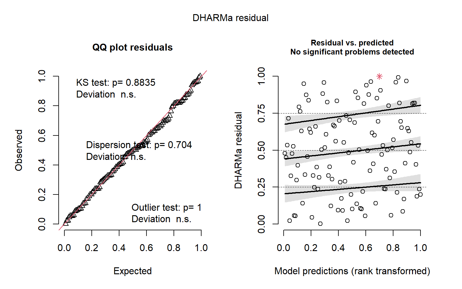
Object of Class DHARMa with simulated residuals based on 250 simulations with refit = FALSE . See ?DHARMa::simulateResiduals for help.

Scaled residual values: 0.7153866 0.001931219 0.696 0.2490446 0.648 0.992 0.1028773 0.5024718 0.3282699 0.8253997 0.4188254 0.3612344 0.8827414 0.1228934 0.6018339 0.236 0.5249315 0.4109765 0.4040863 0.4968128 ...
# native turnover
DHARMa::simulateResiduals(fittedModel = mod_turnover_native, plot = TRUE)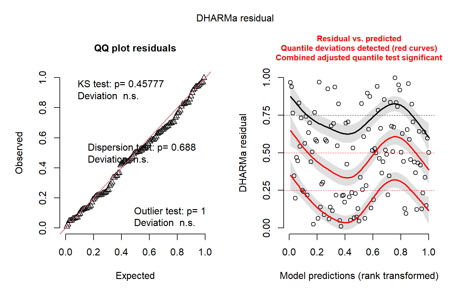
Object of Class DHARMa with simulated residuals based on 250 simulations with refit = FALSE . See ?DHARMa::simulateResiduals for help.

Scaled residual values: 0.3643169 0.9604177 0.218907 0.4996626 0.4468048 0.586672 0.2291625 0.1288934 0.6268271 0.09580275 0.2318073 0.1704958 0.5271945 0.4248068 0.2145687 0.764 0.431788 0.8319357 0.3455402 0.3028504 ...
# NBT turnover
DHARMa::simulateResiduals(fittedModel = mod_turnover_nbt, plot = TRUE)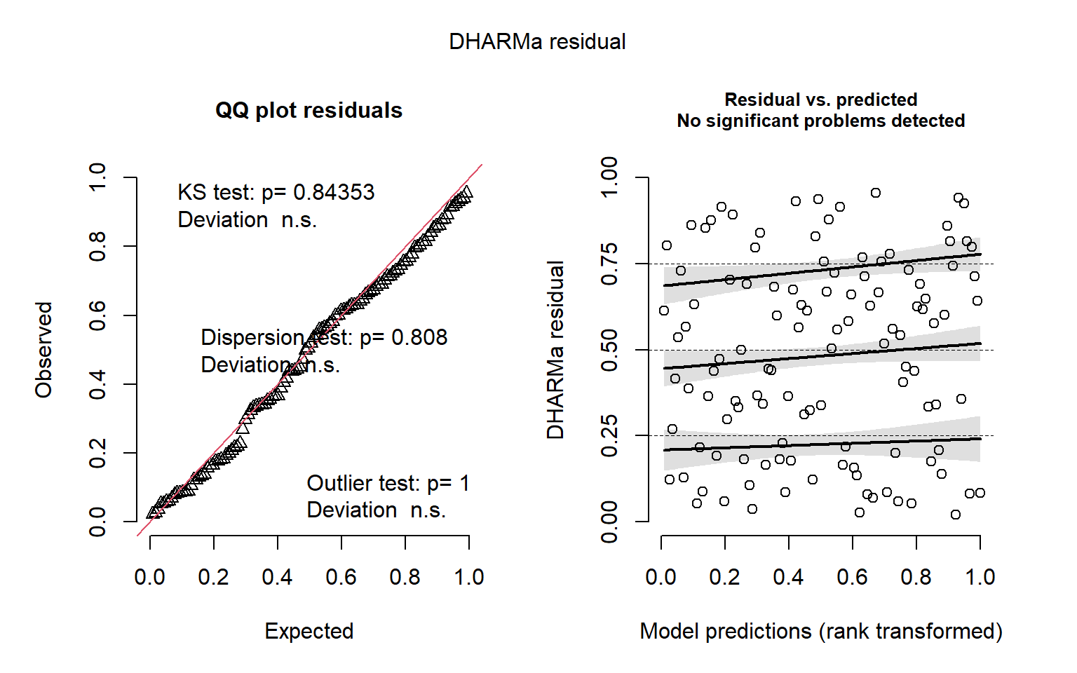
Object of Class DHARMa with simulated residuals based on 250 simulations with refit = FALSE . See ?DHARMa::simulateResiduals for help.

Scaled residual values: 0.8617319 0.5820144 0.2277367 0.2187418 0.208 0.9406471 0.7678828 0.4724905 0.8400271 0.4985776 0.3119429 0.5414365 0.666443 0.4497502 0.1222786 0.6144549 0.05974446 0.8600977 0.084 0.5668753 ...