07 - World map with countries represented by its endemic deficit for non-endemic representation (Figure 2)

07_V_beta_endemics_Fig2.qmd

Plotting endemic deficit and non-endemic representation for each country

Loading packages

#plot
library(ggplot2)
library(patchwork)
library(cowplot)
#map
library(rnaturalearth)
library(rmapshaper)
library(sf)
library(biscale)

Data used

# Data from 02_D_beta-countries.qmd
df_endemic_beta <- readr::read_csv(here::here("data", "processed", "df_endemic_beta.csv"))

Joining metric information with geographical data

countries <- rnaturalearth::ne_countries(returnclass = "sf")

sf_countries <-
  sf::st_as_sf(countries) |>
  dplyr::filter(admin != "Antarctica") |>
  sf::st_transform(crs = "+proj=moll +x_0=0 +y_0=0 +lat_0=0 +lon_0=0") |> 
  dplyr::select(iso_a3_eh)

df_endemic_beta_sf <-
  sf_countries |>
  dplyr::full_join(df_endemic_beta, by = c(iso_a3_eh = "countries"))

First processing spatial data to convert NA values into 0

df_endemic_beta_sf2 <- 
  df_endemic_beta_sf |> 
  sf::st_as_sf() |> 
  rmapshaper::ms_filter_islands(min_area = 12391399903) |> 
  dplyr::mutate(
    type.beta = ifelse(is.na(type.beta), 
                           0, 
                           type.beta),
    native.beta = ifelse(is.na(native.beta), 
                           0, 
                           native.beta))

Create palettes

palette_blue <- colorRampPalette(c("#d3d3d3", "#accaca", "#81c1c1", "#52b6b6"))

palette_pink <- colorRampPalette(c("#d3d3d3", "#c5acc2", "#bb84b1", "#ac5a9c"))

Plotting maps

map_native_endemic_beta <- 
  ggplot() +
  geom_sf(data = df_endemic_beta_sf2,
          aes(geometry = geometry,
              fill = native.beta),
          color = "white",
          size = 0.1, na.rm = T) +
  scale_fill_gradientn(
    colors = palette_pink(10),
    na.value = "#d3d3d3",
    limits = c(0,1)
  )+
  guides(fill = guide_colorbar(
    barheight = unit(0.1, units = "in"),
    barwidth =  unit(4, units = "in"),
    ticks.colour = "grey20",
    title.position="top", 
    title.hjust = 0.5
  )) +
  labs(
    fill = "Endemic deficit"
  )+
  theme_classic()+
  theme(
    legend.position = "bottom",
    legend.margin = margin(-10,0,0,0,"pt"),
    axis.text = element_blank(),  
    axis.ticks = element_blank(),
    axis.line = element_blank()
  ) 

map_type_endemic_beta <- 
  ggplot() +
  geom_sf(data = df_endemic_beta_sf2,
          aes(geometry = geometry,
              fill = type.beta),
          color = "white",
          size = 0.1, na.rm = T) +
  scale_fill_gradientn(
    colors = palette_blue(10),
    na.value = "#d3d3d3",
    limits = c(0,1)
  )+
  guides(fill = guide_colorbar(
    barheight = unit(0.1, units = "in"),
    barwidth =  unit(4, units = "in"),
    ticks.colour = "grey20",
    title.position="top", 
    title.hjust = 0.5
  )) +
  labs(
    fill = "Non-endemic name bearers"
  )+
  theme_classic()+
  theme(
    legend.position = "bottom",
    legend.margin = margin(-10,0,0,0,"pt"),
    axis.text = element_blank(),  
    axis.ticks = element_blank(),
    axis.line = element_blank()
  ) 

Plotting the two quantities in a bivariate map

sf_bivar_types_endemic <-
  bi_class(df_endemic_beta_sf2, 
           x = type.beta, 
           y = native.beta, 
           style = "equal",
           dim = 4)

bivar_map_types_endemic <- 
  ggplot() +
  geom_sf(data = sf_bivar_types_endemic, 
          aes(geometry = geometry,
              fill = bi_class), 
          color = "white",
          size = 0.1, 
          show.legend = FALSE) +
  bi_scale_fill(pal = "DkBlue2", 
                dim = 4) +
  theme_classic()+
  theme(
    legend.position = "bottom",
    legend.title = element_blank(),
        axis.text = element_blank(),  
        axis.ticks = element_blank(),
        axis.line = element_blank(),
    panel.background = element_rect(fill = NA),
    plot.background = element_rect(fill = NA)
  ) 

legend <-
  bi_legend(pal = "DkBlue2",
            dim = 4,
            xlab = "Non endemic",
            ylab = "Endemic",
            size = )

bivar_map_type_final_endemic <- 
  ggdraw() +
  draw_plot(legend, 0.0, 0.15, 0.25, 0.25) +
  draw_plot(bivar_map_types_endemic, 0, 0, 1, 1)

Joining all the maps

map_turnover_endemic <-
  map_native_endemic_beta+map_type_endemic_beta+bivar_map_type_final_endemic+
  patchwork::plot_layout(
    design = 
"AB
 CC"
  )+
  patchwork::plot_annotation(tag_levels = "a")&
  theme(
    plot.tag = element_text(face = "bold", hjust = 0, vjust = 1),
    plot.tag.position = c(0, 1),
  )

map_turnover_endemic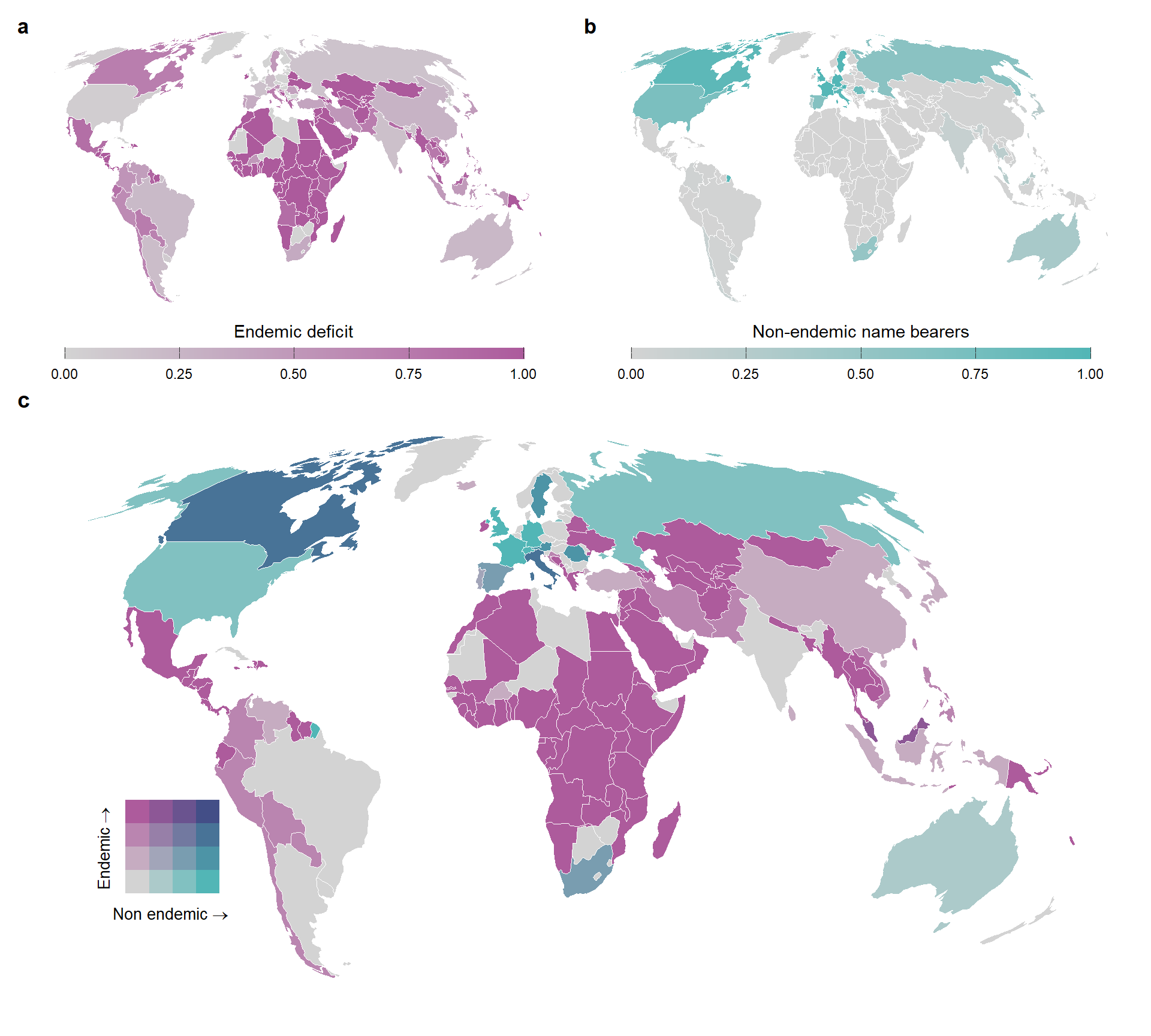

ggsave(here::here("output", "figures", "Fig2_turnover_metrics_endemics.png"),
       map_turnover_endemic, dpi=600, width = 10, height = 9)