Computing evoregions analysis • Herodotools

This article outlines the basic workflow for constructing evoregions, starting from defining the maximum number of clusters to the visualization of the final results generated by the evoregion() function. The workflow is organized into two main sections:

Setting the maximum number of clusters to be considered in the evoregion analysis.
Computing evoregions using the number of clusters that yields the most stable and interpretable solution in the analysis.

Setting the maximum number of clusters

In the evoregion workflow, defining the maximum number of clusters to be tested is a key step. This is particularly important because the find.clusters() function from the {adegenet} package is sensitive to this parameter: different values of the maximum number of clusters may lead to different group assignments.

The purpose of the find_max_nclust() function in {Herodotools} is to identify the maximum number of clusters that produces the most stable grouping solution. To do this, the function runs find.clusters() multiple times across a range of maximum cluster values and evaluates the consistency of the resulting solutions.

Stability is assessed by computing the correlation between clustering results across runs, combined with different tolerance values for the confidence.level argument. The optimal maximum number of clusters is the one that maximizes this correlation, serving as a proxy for the stability of the evoregion solution.

In this tutorial, we use example data provided in the {Herodotools} package. The akodon_site dataset represents the occurrence of species across assemblages mapped in 1° × 1° grid cells. The akodon_newick object contains the phylogenetic tree (in Newick format) describing the evolutionary relationships among species of the tribe Akodontini.

library(Herodotools)
data("akodon_sites")
data("akodon_newick")

# minor data processing 

site_xy <- akodon_sites  |>  
  dplyr::select(LONG, LAT) 

akodon_pa <- akodon_sites |> 
  dplyr::select(-LONG, -LAT)

spp_in_tree <- names(akodon_pa) %in% akodon_newick$tip.label
akodon_pa_tree <- akodon_pa[, spp_in_tree]

First, we need to compute the Principal Component of Phylogenetic Structure (PCPS) matrix, which will be used as input for the find_max_nclust() function. This can be done using the pcps() function from the {PCPS} package.

pcps_bray <-
  PCPS::pcps(akodon_pa_tree, phylodist = cophenetic(akodon_newick), method = "bray")

values_bray <- pcps_bray$values # PCPS eigenvalues, relative eigenvalues and cumulative relative eigenvalues

# Define a threshold value for eigenvectors (eigenvectors containing more than 5% of variation)
thresh_bray <- max(which(values_bray[, 2] >= 0.05))
vec_bray <- pcps_bray$vectors # eigenvectors

Now we can estimate the optimal maximum number of groups using the find_max_nclust() function implemented in {Herodotools}. This function supports parallel computation via the {future} package. We recomend to set the parallel backend using future::plan() first.

# setting function to work in parallel according to user settings
library(future)
library(progressr)

# Detect safe max cores
ncores <- future::availableCores()  # dynamic
safety_margin <- 1
workers <- max(1, ncores - safety_margin)

plan(multisession, workers = workers) this 
future::plan(sequential)
handlers(global = TRUE)
handlers("txtprogressbar")   # terminal progress bar + timing info

Then, run the find_max_clust function


matrix_optimal_maxclust <- 
  find_max_nclust(x = vec_bray,
                  threshold = thresh_bray, 
                  max.nclust = c(3, 4, 5, 7, 9, 10),
                  nperm = 300, 
                  method = "kmeans", 
                  stat = "BIC", 
                  criterion = "diffNgroup",
                  subset = 100,
                  confidence.level = c(0.7, 0.8, 0.9, 0.95, 0.99))
#> Warning: UNRELIABLE VALUE: One of the 'future.apply' iterations
#> ('future_lapply-1') unexpectedly generated random numbers without declaring so.
#> There is a risk that those random numbers are not statistically sound and the
#> overall results might be invalid. To fix this, specify 'future.seed=TRUE'. This
#> ensures that proper, parallel-safe random numbers are produced via a parallel
#> RNG method. To disable this check, use 'future.seed = NULL', or set option
#> 'future.rng.onMisuse' to "ignore".
#> Warning: UNRELIABLE VALUE: One of the 'future.apply' iterations
#> ('future_lapply-1') unexpectedly generated random numbers without declaring so.
#> There is a risk that those random numbers are not statistically sound and the
#> overall results might be invalid. To fix this, specify 'future.seed=TRUE'. This
#> ensures that proper, parallel-safe random numbers are produced via a parallel
#> RNG method. To disable this check, use 'future.seed = NULL', or set option
#> 'future.rng.onMisuse' to "ignore".
#> Warning: UNRELIABLE VALUE: One of the 'future.apply' iterations
#> ('future_lapply-1') unexpectedly generated random numbers without declaring so.
#> There is a risk that those random numbers are not statistically sound and the
#> overall results might be invalid. To fix this, specify 'future.seed=TRUE'. This
#> ensures that proper, parallel-safe random numbers are produced via a parallel
#> RNG method. To disable this check, use 'future.seed = NULL', or set option
#> 'future.rng.onMisuse' to "ignore".
#> Warning: Quick-TRANSfer stage steps exceeded maximum (= 36600)
#> Warning: UNRELIABLE VALUE: One of the 'future.apply' iterations
#> ('future_lapply-1') unexpectedly generated random numbers without declaring so.
#> There is a risk that those random numbers are not statistically sound and the
#> overall results might be invalid. To fix this, specify 'future.seed=TRUE'. This
#> ensures that proper, parallel-safe random numbers are produced via a parallel
#> RNG method. To disable this check, use 'future.seed = NULL', or set option
#> 'future.rng.onMisuse' to "ignore".
#> Warning: Quick-TRANSfer stage steps exceeded maximum (= 36600)
#> Warning: Quick-TRANSfer stage steps exceeded maximum (= 36600)
#> Warning: Quick-TRANSfer stage steps exceeded maximum (= 36600)
#> Warning: Quick-TRANSfer stage steps exceeded maximum (= 36600)
#> Warning: Quick-TRANSfer stage steps exceeded maximum (= 36600)
#> Warning: Quick-TRANSfer stage steps exceeded maximum (= 36600)
#> Warning: Quick-TRANSfer stage steps exceeded maximum (= 36600)
#> Warning: Quick-TRANSfer stage steps exceeded maximum (= 36600)
#> Warning: Quick-TRANSfer stage steps exceeded maximum (= 36600)
#> Warning: Quick-TRANSfer stage steps exceeded maximum (= 36600)
#> Warning: Quick-TRANSfer stage steps exceeded maximum (= 36600)
#> Warning: Quick-TRANSfer stage steps exceeded maximum (= 36600)
#> Warning: did not converge in 100000 iterations
#> Warning: Quick-TRANSfer stage steps exceeded maximum (= 36600)
#> Warning: UNRELIABLE VALUE: One of the 'future.apply' iterations
#> ('future_lapply-1') unexpectedly generated random numbers without declaring so.
#> There is a risk that those random numbers are not statistically sound and the
#> overall results might be invalid. To fix this, specify 'future.seed=TRUE'. This
#> ensures that proper, parallel-safe random numbers are produced via a parallel
#> RNG method. To disable this check, use 'future.seed = NULL', or set option
#> 'future.rng.onMisuse' to "ignore".
#> Warning: Quick-TRANSfer stage steps exceeded maximum (= 36600)
#> Warning: Quick-TRANSfer stage steps exceeded maximum (= 36600)
#> Warning: Quick-TRANSfer stage steps exceeded maximum (= 36600)
#> Warning: Quick-TRANSfer stage steps exceeded maximum (= 36600)
#> Warning: did not converge in 100000 iterations
#> Warning: Quick-TRANSfer stage steps exceeded maximum (= 36600)
#> Warning: did not converge in 100000 iterations
#> Warning: Quick-TRANSfer stage steps exceeded maximum (= 36600)
#> Warning: Quick-TRANSfer stage steps exceeded maximum (= 36600)
#> Warning: did not converge in 100000 iterations
#> Warning: Quick-TRANSfer stage steps exceeded maximum (= 36600)
#> Warning: did not converge in 100000 iterations
#> Warning: Quick-TRANSfer stage steps exceeded maximum (= 36600)
#> Warning: Quick-TRANSfer stage steps exceeded maximum (= 36600)
#> Warning: Quick-TRANSfer stage steps exceeded maximum (= 36600)
#> Warning: Quick-TRANSfer stage steps exceeded maximum (= 36600)
#> Warning: did not converge in 100000 iterations
#> Warning: Quick-TRANSfer stage steps exceeded maximum (= 36600)
#> Warning: Quick-TRANSfer stage steps exceeded maximum (= 36600)
#> Warning: UNRELIABLE VALUE: One of the 'future.apply' iterations
#> ('future_lapply-1') unexpectedly generated random numbers without declaring so.
#> There is a risk that those random numbers are not statistically sound and the
#> overall results might be invalid. To fix this, specify 'future.seed=TRUE'. This
#> ensures that proper, parallel-safe random numbers are produced via a parallel
#> RNG method. To disable this check, use 'future.seed = NULL', or set option
#> 'future.rng.onMisuse' to "ignore".

This matrix summarizes the results of the analysis of stability of cluster computation for different values of the maximum number of groups. Each row corresponds to a tested number of groups and contains the associated confidence level. The confidence level represents the proportion of correlation values that are equal to or greater than the threshold being evaluated. Values closer to 1 indicate a higher stability of the clustering solution for that number of groups under the specified confidence level. In other words, values approaching 1 suggest that a given number of groups yields consistent and reliable cluster structures.

In this example, the maximum number of groups that yields the most stable solution is 3. Therefore, we use this value in the evoregion() computation that follows.

Computing evoregions

Here we use the function calc_evoregion, originally described in Maestri and Duarte (2020) and implemented in the {Herodotools} package. This classification method performs a biogeographical regionalization based on a phylogenetic fuzzy matrix, combined with a Discriminant Analysis of Principal Components (DAPC) using k-means clustering. Evoregions represent areas that correspond to centers of lineage diversification, reflecting historical evolutionary radiations within clades (Maestri & Duarte, 2020).

To compute evoregions, the user must provide a species occurrence matrix and a phylogenetic tree. If max.n.clust is not specified, the evoregion() function automatically selects the maximum number of clusters using the “elbow” method, as implemented in the {phyloregion} package (https://besjournals.onlinelibrary.wiley.com/doi/epdf/10.1111/2041-210X.13478).

However, we strongly recommend using the find_max_nclust() function to determine the maximum number of clusters, as demonstrated in the previous section. This approach identifies the most stable clustering solution and is therefore more aligned with the methodological rationale of the evoregion framework.

The seed argument ensures reproducibility: if the analysis is repeated with the same data and argument settings, the same numerical labels are assigned to the groups. Without setting a seed, the group labels (i.e., the cluster numbers) may differ across runs even when the grouping structure remains the same.

Here, we set max.n.clust = 3, based on the result obtained in the previous step.

regions <- 
  Herodotools::calc_evoregions(
  comm = akodon_pa_tree,
  phy = akodon_newick, 
  seed = 100, max.n.clust = 3
  )

site_region <- regions$cluster_evoregions # this is the classification result for each site

We can plot the regions in the map

evoregion_df <- data.frame(
  site_xy, 
  site_region
)

r_evoregion <- terra::rast(evoregion_df)

# Converting evoregion to a spatial polygon data frame, so it can be plotted
sf_evoregion <- terra::as.polygons(r_evoregion) |> 
  sf::st_as_sf()


# Downloading coastline continents and croping to keep only South America
coastline <- rnaturalearth::ne_coastline(returnclass = "sf")
map_limits <- list(
  x = c(-95, -30),
  y = c(-55, 12)
)

# Assigning the same projection to both spatial objects
sf::st_crs(sf_evoregion) <- sf::st_crs(coastline)

# Colours to plot evoregions
col_two_hues <- c(
  "#3d291a",
  "#fcc573"
)

Finally, plotting evoregions in the map

library(ggplot2)
map_evoregion <- 
  evoregion_df |> 
  ggplot2::ggplot() + 
  ggplot2::geom_raster(ggplot2::aes(x = LONG, y = LAT, fill = site_region)) + 
  ggplot2::scale_fill_manual(
    name = "", 
    labels = LETTERS[1:5],
    values = rev(col_two_hues)
  ) +
  ggplot2::geom_sf(data = coastline) +
  ggplot2::geom_sf(
    data = sf_evoregion, 
    color = "#040400",
    fill = NA, 
    size = 0.2) +
  ggplot2::coord_sf(xlim = map_limits$x, ylim = map_limits$y) +
  ggplot2::ggtitle("") + 
  ggplot2::theme_bw() +
  ggplot2::xlab("Longitude") +
  ggplot2::ylab("Latitude") +
  ggplot2::theme(
        legend.position = "bottom",
        plot.margin = unit(c(0.1, 0.1, 0.1, 0.1), "mm"),
        legend.text = element_text(size = 12), 
        axis.text = element_text(size = 7),
        axis.title.x = element_text(size = 11),
        axis.title.y = element_text(size = 11)
        )

map_evoregion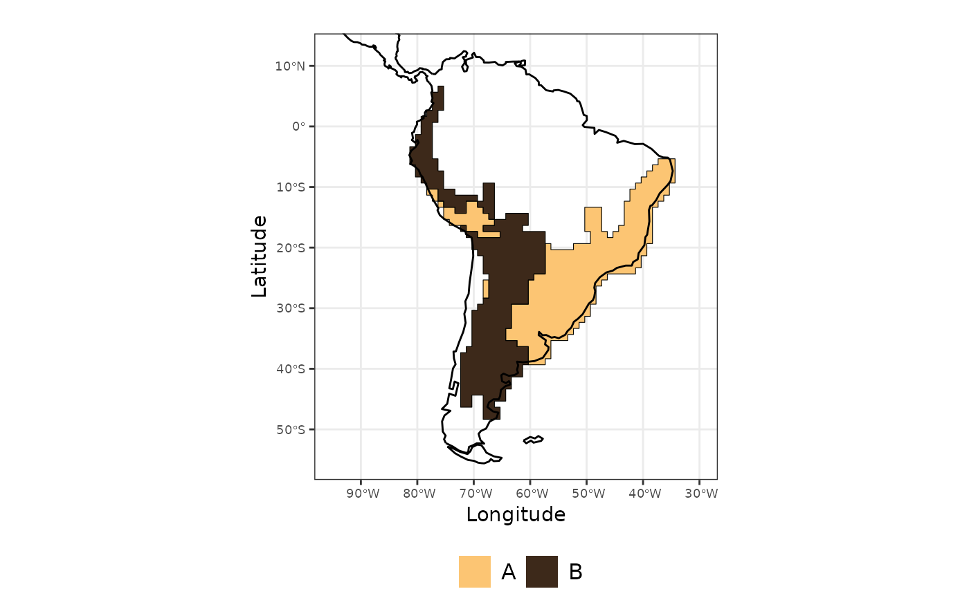

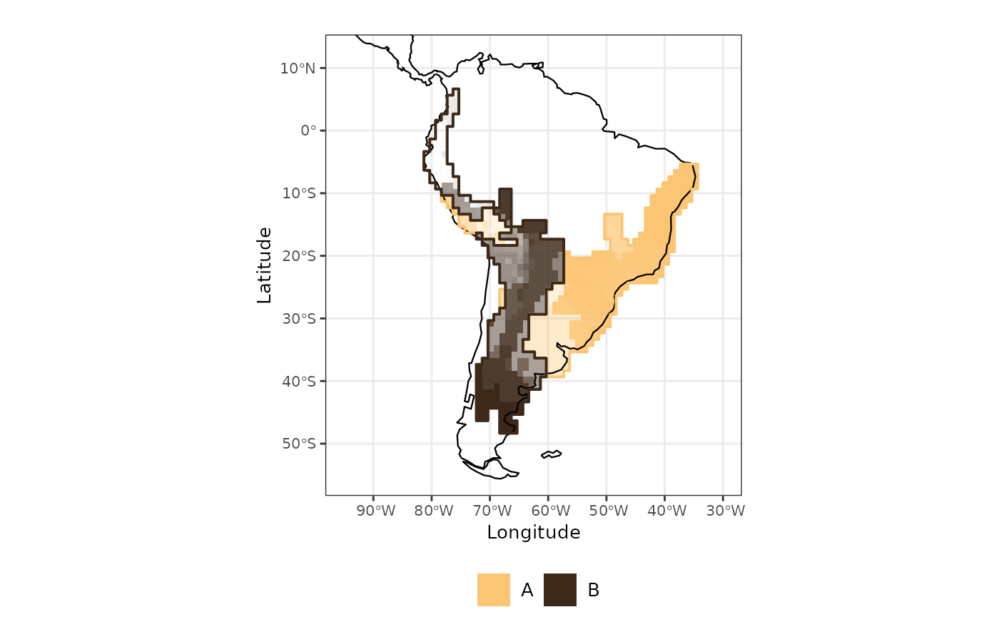
The output from evoregion() indicates the presence of two distinct regions. However, not all cells share the same degree of affiliation with the region to which they were assigned. Cells with high affiliation values represent assemblages that are highly similar to other cells within the same region. Conversely, cells with low affiliation values correspond to areas with high turnover, that is, areas where multiple colonization events by different lineages have occurred (Maestri & Duarte, 2020).

We can calculate the affiliation of each cell to its corresponding region with the function calc_affiliation_evoreg


# distance matrix using 4 significant PCPS axis accordingly to the 5% threshold 
dist_phylo_PCPS <- vegan::vegdist(vec_bray[, 1:thresh_bray], method = "euclidean")

# calculating affiliation values for each assemblage 
afi <- calc_affiliation_evoreg(phylo.comp.dist = dist_phylo_PCPS,
                          groups = site_region) 

# binding the information in a data frame
sites <- dplyr::bind_cols(site_xy, site_region =  site_region, afi)

Now we can map the evoregions along with the degree of affiliation for each cell. The affiliation values are represented by the intensity of the colors: cells with high affiliation appear in strong, saturated colors, while cells with low affiliation are shown in more faded colors. In other words, the more faded a cell’s color, the weaker its affiliation to the assigned evoregion.

map_joint_evoregion_afilliation <- 
   evoregion_df %>% 
   ggplot() + 
   ggplot2::geom_raster(ggplot2::aes(x = LONG, y = LAT, fill = site_region), 
               alpha = sites[, "afilliation"]) + 
   ggplot2::scale_fill_manual(
     name = "", 
     labels = LETTERS[1:2],
     values = rev(col_two_hues)
   ) +
   ggplot2::geom_sf(data = coastline, size = 0.4) +
   ggplot2::geom_sf(
     data = sf_evoregion, 
     color = rev(col_two_hues),
     fill = NA, 
     size = 0.7) +
   ggplot2::coord_sf(xlim = map_limits$x, ylim = map_limits$y) +
   ggplot2::ggtitle("") + 
   guides(guide_legend(direction = "vertical")) +
   ggplot2::theme_bw() +
  ggplot2::xlab("Longitude") +
  ggplot2::ylab("Latitude") +
  ggplot2::theme(
        legend.position = "bottom",
        plot.margin = unit(c(0.1, 0.1, 0.1, 0.1), "mm"),
        legend.text = element_text(size = 10), 
        axis.text = element_text(size = 8),
        axis.title.x = element_text(size = 10),
        axis.title.y = element_text(size = 10)
        )
#> Warning: Guides provided to `guides()` must be named.
#> ℹ All guides are unnamed.

map_joint_evoregion_afilliation