Time series metrics
time-series-metrics.Rmd
library(ggplot2)
library(dplyr)
#>
#> Attaching package: 'dplyr'
#> The following objects are masked from 'package:stats':
#>
#>     filter, lag
#> The following objects are masked from 'package:base':
#>
#>     intersect, setdiff, setequal, union
library(Buccaneer)
Background
In this article we will show how to calculate different metrics of
interspecific competition (or sometimes coexistence metrics) at
different taxonomic levels and spatial scales in deep time using
{Buccaneer} R package.
For all metrics we will use data from Graciotti et al. (2025). The data comprises
fossil record of North American canids, a group that has been well
caracterized ecologically and regarding fossil record. This data is also
part of the {Buccaneer} package and is comprised by:
Species longevity: A data frame describing the Origination Time (TS) and Extinction Time (TE) obtained with Bayesian framework called PyRate
Occurrence record data: A data frame with fossil occurrence records retrieved from Paleobiology Database including only North American canids. For details in data process and curatorial work check out Graciotti et al. (2025)
Species traits: A data frame with ecomorphological characterization of species with traits that present important proxies for determining species niches. For downstream analysis we use mostly body mass and LDA to infer diet of species. For details on how this data was computed see Graciotti et al. (2025)
Loading data and packages
In the following examples, we will use three datasets that are
embedded in the Buccaneer package and can be loaded as
follows:
Interspecific competition at clade level
At this section we present metrics to calculate proxy metrics that represent interspecific competition at clade level. By competition at clade level we mean the competition described by the variation in the absolute number of coexisting species or by how the morphospace occupation change through time. We perform this characterization at different scales:
- Regional: Considering all species present at a given time slice as
    coexisting species

- Local (or Site): We consider a coexistence only species present at the
    same timeslice and spatial area.

- Reach: A coexistence is considered only when the potential dispersion
   threshold distance in space between a pair of species is satisfied.
   For more details in reach criteria see @graciotti_ecological_2025
Regional scale
Calculating time series at clade level and regional scale
res_clade_regional <-
  clade_regional_coexistence(df.TS.TE = df_longevities_canidae,
                             time.slice = 0.1,
                             round.digits = 10,
                             species = "species",
                             TS = "TS",
                             TE = "TE")
Here we calculate the mean distances using a general function that
allows to set up the group comparison in which the mean will be
calculate. It can be between to calculate mean distances
between a focal and a target group or within to calculate
the mean trait distance only within the focal group. To this end we will
use the diet_cat column of the trait_canidae
data frame, that contains a
classification of canidae species in two categories: hypercarnivores and
mesocarnivores.
First we need to join this information to the
df_longvities_canidae data frame
df_longevities_canidae_trait <-
  df_longevities_canidae |>
  left_join(traits_canidae, by = "species")
This function is also a general solution to calculate the mean trait
distance using different number of species/genus that are close to each
other. To set up the number of closest species that will be used in the
calculation of mean pairwise distances we will change the argument
nearest.taxon. 1 is equivalent of mean nearest distance and
all corresponds to the calculation of mean pairwise
distance (mpd) using all coexisting species.
The next chunk of code show an example on how we can calculate mean distances in the morphospace using different types of comparisons and varying the number of closest species in the morphospace considered in the calculation
ld1 <- traits_canidae$LD1
names(ld1) <- traits_canidae$species
dist_body_mass <- dist(ld1) # computing pairwise distance matrix for body mass

# distances between groups using diet category
res_regional_mnd_between <-
  clade_regional_distance(df.TS.TE = df_longevities_canidae_trait,
                          time.slice = 0.1,
                          dist.trait = dist_body_mass,
                          nearest.taxon = 1,
                          round.digits = 1,
                          species = "species",
                          TS = "TS",
                          TE = "TE",
                          group = "diet_cat",
                          group.focal.compare = c("meso", "hyper"),
                          type.comparison = "between")


# distance in morphospace computed within the focal group, in this case is mesocarnivores
res_regional_mnd_within <-
  clade_regional_distance(df.TS.TE = df_longevities_canidae_trait,
                          time.slice = 0.1,
                          dist.trait = dist_body_mass,
                          nearest.taxon = 1,
                          round.digits = 1,
                          species = "species",
                          TS = "TS",
                          TE = "TE",
                          group = "diet_cat",
                          group.focal.compare = c("meso", "meso"),
                          type.comparison = "within")
Let’s check out the results of these two competition metrics. First we need to join the results to plot in one graphic
all_mnd_regional <- rbind(res_regional_mnd_between, res_regional_mnd_within)
all_mnd_regional2 <-
  data.frame(all_mnd_regional,
             group_res = rep(c("Between", "Within"),
                             each = nrow(res_regional_mnd_within))
  )
Plotting the results
res_clade_regional |>
  mutate(time.slice = as.numeric(time.slice)) |>
  ggplot(aes(x = time.slice, y = coexistence)) +
  geom_smooth(
    se = TRUE,
    method = "loess",
    linewidth = 0.6
  ) +
  geom_line(
    linewidth = 0.4
  ) +
  labs(
    x = "Time (Ma)",
    y = "Coexistence"
  ) +
  scale_x_reverse(
    breaks = seq(
      from = 0,
      to   = max(res_clade_regional$time.slice, na.rm = TRUE),
      by   = 5
    )
  ) +
  theme_minimal(base_size = 10) +
  theme(
    legend.position = "none",
    axis.line = element_line(color = "black", linewidth = 0.4),
    axis.title = element_text(size = 9),
    axis.text  = element_text(size = 7),
    axis.title.x = element_text(size = 9),
    axis.title.y = element_text(size = 9),
    panel.grid.minor = element_blank()
  )
#> `geom_smooth()` using formula = 'y ~ x'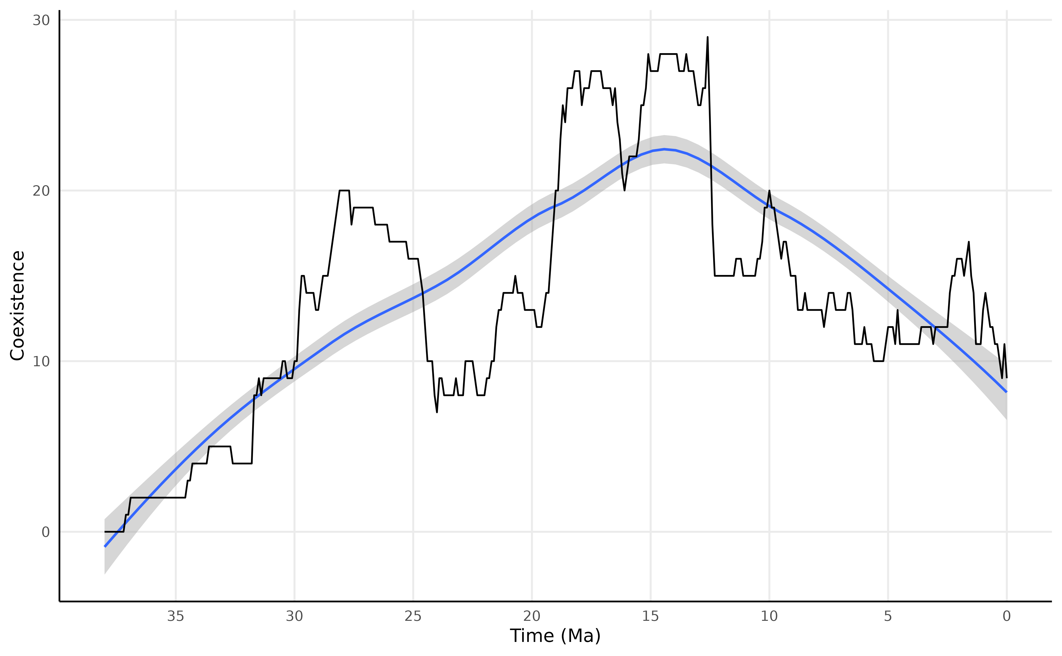
Site scale
res_clade_site <-
  clade_site_coexistence(df.TS.TE = df_longevities_canidae,
                         df.occ = df_occurrence_canidae,
                         time.slice = 0.1,
                         round.digits = 1,
                         species = "species",
                         TS = "TS",
                         TE = "TE",
                         Max.age = "max_T",
                         Min.age = "min_T",
                         site = "site.char")
Plotting the results
res_clade_site |>
  ggplot(aes(x = as.numeric(time.slice), y = mean.coexistence)) +
  geom_line(aes(x = as.numeric(time.slice), y = mean.coexistence)) +
  geom_smooth(se = TRUE, method = "loess", size = 1) +  # Line thickness for better visibility
  labs(title = "",
       x = "Time (Ma)",
       y = "Mean site coexistence") +
  scale_x_continuous(breaks = seq(max(as.numeric(res_clade_site$time.slice)), 0, by = -10)) +
  scale_x_reverse() +
  theme_minimal(base_size = 10) +
  theme(
    legend.position = "none",
    axis.line = element_line(color = "black", linewidth = 0.4),
    axis.title = element_text(size = 9),
    axis.text  = element_text(size = 7),
    axis.title.x = element_text(size = 9),
    axis.title.y = element_text(size = 9),
    panel.grid.minor = element_blank()
  )
We can also calculate the distance in morphospace using site criteria
res_clade_site_distance <-
  clade_site_distance(df.TS.TE = df_longevities_canidae,
                      df.occ = df_occurrence_canidae,
                      time.slice = 0.1,
                      round.digits = 1,
                      dist.trait = dist_body_mass,
                      nearest.taxon = 1,
                      species = "species",
                      TS = "TS",
                      TE = "TE",
                      Max.age = "max_T",
                      Min.age = "min_T",
                      site = "site.char")

# calculating between mesocarnivores and hypercarnivores species
res_clade_site_distance_between <-
  clade_site_distance(df.TS.TE = df_longevities_canidae_trait,
                      df.occ = df_occurrence_canidae,
                      time.slice = 0.1,
                      round.digits = 1,
                      dist.trait = dist_body_mass,
                      nearest.taxon = 1,
                      group = "diet_cat",
                      group.focal.compare = c("meso", "hyper"),
                      type.comparison = "between",
                      species = "species",
                      TS = "TS",
                      TE = "TE",
                      Max.age = "max_T",
                      Min.age = "min_T",
                      site = "site.char")
#> Warning in mean.default(x, na.rm = TRUE): argument is not numeric or logical:
#> returning NA
#> Warning in mean.default(x, na.rm = TRUE): argument is not numeric or logical:
#> returning NA
#> Warning in mean.default(x, na.rm = TRUE): argument is not numeric or logical:
#> returning NA
#> Warning in mean.default(x, na.rm = TRUE): argument is not numeric or logical:
#> returning NA
#> Warning in mean.default(x, na.rm = TRUE): argument is not numeric or logical:
#> returning NA
#> Warning in mean.default(x, na.rm = TRUE): argument is not numeric or logical:
#> returning NA
#> Warning in mean.default(x, na.rm = TRUE): argument is not numeric or logical:
#> returning NA
#> Warning in mean.default(x, na.rm = TRUE): argument is not numeric or logical:
#> returning NA
#> Warning in mean.default(x, na.rm = TRUE): argument is not numeric or logical:
#> returning NA
#> Warning in mean.default(x, na.rm = TRUE): argument is not numeric or logical:
#> returning NA
#> Warning in mean.default(x, na.rm = TRUE): argument is not numeric or logical:
#> returning NA
#> Warning in mean.default(x, na.rm = TRUE): argument is not numeric or logical:
#> returning NA
#> Warning in mean.default(x, na.rm = TRUE): argument is not numeric or logical:
#> returning NA
#> Warning in mean.default(x, na.rm = TRUE): argument is not numeric or logical:
#> returning NA
#> Warning in mean.default(x, na.rm = TRUE): argument is not numeric or logical:
#> returning NA
#> Warning in mean.default(x, na.rm = TRUE): argument is not numeric or logical:
#> returning NA
#> Warning in mean.default(x, na.rm = TRUE): argument is not numeric or logical:
#> returning NA
#> Warning in mean.default(x, na.rm = TRUE): argument is not numeric or logical:
#> returning NA
#> Warning in mean.default(x, na.rm = TRUE): argument is not numeric or logical:
#> returning NA
#> Warning in mean.default(x, na.rm = TRUE): argument is not numeric or logical:
#> returning NA
#> Warning in mean.default(x, na.rm = TRUE): argument is not numeric or logical:
#> returning NA
#> Warning in mean.default(x, na.rm = TRUE): argument is not numeric or logical:
#> returning NA
#> Warning in mean.default(x, na.rm = TRUE): argument is not numeric or logical:
#> returning NA
#> Warning in mean.default(x, na.rm = TRUE): argument is not numeric or logical:
#> returning NA
#> Warning in mean.default(x, na.rm = TRUE): argument is not numeric or logical:
#> returning NA
#> Warning in mean.default(x, na.rm = TRUE): argument is not numeric or logical:
#> returning NA
#> Warning in mean.default(x, na.rm = TRUE): argument is not numeric or logical:
#> returning NA
#> Warning in mean.default(x, na.rm = TRUE): argument is not numeric or logical:
#> returning NA
#> Warning in mean.default(x, na.rm = TRUE): argument is not numeric or logical:
#> returning NA
#> Warning in mean.default(x, na.rm = TRUE): argument is not numeric or logical:
#> returning NA
#> Warning in mean.default(x, na.rm = TRUE): argument is not numeric or logical:
#> returning NA
#> Warning in mean.default(x, na.rm = TRUE): argument is not numeric or logical:
#> returning NA
#> Warning in mean.default(x, na.rm = TRUE): argument is not numeric or logical:
#> returning NA
#> Warning in mean.default(x, na.rm = TRUE): argument is not numeric or logical:
#> returning NA
#> Warning in mean.default(x, na.rm = TRUE): argument is not numeric or logical:
#> returning NA
#> Warning in mean.default(x, na.rm = TRUE): argument is not numeric or logical:
#> returning NA
#> Warning in mean.default(x, na.rm = TRUE): argument is not numeric or logical:
#> returning NA
#> Warning in mean.default(x, na.rm = TRUE): argument is not numeric or logical:
#> returning NA
#> Warning in mean.default(x, na.rm = TRUE): argument is not numeric or logical:
#> returning NA
#> Warning in mean.default(x, na.rm = TRUE): argument is not numeric or logical:
#> returning NA
#> Warning in mean.default(x, na.rm = TRUE): argument is not numeric or logical:
#> returning NA
#> Warning in mean.default(x, na.rm = TRUE): argument is not numeric or logical:
#> returning NA
#> Warning in mean.default(x, na.rm = TRUE): argument is not numeric or logical:
#> returning NA
#> Warning in mean.default(x, na.rm = TRUE): argument is not numeric or logical:
#> returning NA
#> Warning in mean.default(x, na.rm = TRUE): argument is not numeric or logical:
#> returning NA
#> Warning in mean.default(x, na.rm = TRUE): argument is not numeric or logical:
#> returning NA
#> Warning in mean.default(x, na.rm = TRUE): argument is not numeric or logical:
#> returning NA
#> Warning in mean.default(x, na.rm = TRUE): argument is not numeric or logical:
#> returning NA
#> Warning in mean.default(x, na.rm = TRUE): argument is not numeric or logical:
#> returning NA
#> Warning in mean.default(x, na.rm = TRUE): argument is not numeric or logical:
#> returning NA
#> Warning in mean.default(x, na.rm = TRUE): argument is not numeric or logical:
#> returning NA
#> Warning in mean.default(x, na.rm = TRUE): argument is not numeric or logical:
#> returning NA
#> Warning in mean.default(x, na.rm = TRUE): argument is not numeric or logical:
#> returning NA
#> Warning in mean.default(x, na.rm = TRUE): argument is not numeric or logical:
#> returning NA
#> Warning in mean.default(x, na.rm = TRUE): argument is not numeric or logical:
#> returning NA
#> Warning in var(x, na.rm = TRUE): NAs introduced by coercion
#> Warning in var(x, na.rm = TRUE): NAs introduced by coercion
#> Warning in var(x, na.rm = TRUE): NAs introduced by coercion
#> Warning in var(x, na.rm = TRUE): NAs introduced by coercion
#> Warning in var(x, na.rm = TRUE): NAs introduced by coercion
#> Warning in var(x, na.rm = TRUE): NAs introduced by coercion
#> Warning in var(x, na.rm = TRUE): NAs introduced by coercion
#> Warning in var(x, na.rm = TRUE): NAs introduced by coercion
#> Warning in var(x, na.rm = TRUE): NAs introduced by coercion
#> Warning in var(x, na.rm = TRUE): NAs introduced by coercion
#> Warning in var(x, na.rm = TRUE): NAs introduced by coercion
#> Warning in var(x, na.rm = TRUE): NAs introduced by coercion
#> Warning in var(x, na.rm = TRUE): NAs introduced by coercion
#> Warning in var(x, na.rm = TRUE): NAs introduced by coercion
#> Warning in var(x, na.rm = TRUE): NAs introduced by coercion
#> Warning in var(x, na.rm = TRUE): NAs introduced by coercion
#> Warning in var(x, na.rm = TRUE): NAs introduced by coercion
#> Warning in var(x, na.rm = TRUE): NAs introduced by coercion
#> Warning in var(x, na.rm = TRUE): NAs introduced by coercion
#> Warning in var(x, na.rm = TRUE): NAs introduced by coercion
#> Warning in var(x, na.rm = TRUE): NAs introduced by coercion
#> Warning in var(x, na.rm = TRUE): NAs introduced by coercion
#> Warning in var(x, na.rm = TRUE): NAs introduced by coercion
#> Warning in var(x, na.rm = TRUE): NAs introduced by coercion
#> Warning in var(x, na.rm = TRUE): NAs introduced by coercion
#> Warning in var(x, na.rm = TRUE): NAs introduced by coercion
#> Warning in var(x, na.rm = TRUE): NAs introduced by coercion
#> Warning in var(x, na.rm = TRUE): NAs introduced by coercion
#> Warning in var(x, na.rm = TRUE): NAs introduced by coercion
#> Warning in var(x, na.rm = TRUE): NAs introduced by coercion
#> Warning in var(x, na.rm = TRUE): NAs introduced by coercion
#> Warning in var(x, na.rm = TRUE): NAs introduced by coercion
#> Warning in var(x, na.rm = TRUE): NAs introduced by coercion
#> Warning in var(x, na.rm = TRUE): NAs introduced by coercion
#> Warning in var(x, na.rm = TRUE): NAs introduced by coercion
#> Warning in var(x, na.rm = TRUE): NAs introduced by coercion
#> Warning in var(x, na.rm = TRUE): NAs introduced by coercion
#> Warning in var(x, na.rm = TRUE): NAs introduced by coercion
#> Warning in var(x, na.rm = TRUE): NAs introduced by coercion
#> Warning in var(x, na.rm = TRUE): NAs introduced by coercion
#> Warning in var(x, na.rm = TRUE): NAs introduced by coercion
#> Warning in var(x, na.rm = TRUE): NAs introduced by coercion
#> Warning in var(x, na.rm = TRUE): NAs introduced by coercion
#> Warning in var(x, na.rm = TRUE): NAs introduced by coercion
#> Warning in var(x, na.rm = TRUE): NAs introduced by coercion
#> Warning in var(x, na.rm = TRUE): NAs introduced by coercion
#> Warning in var(x, na.rm = TRUE): NAs introduced by coercion
#> Warning in var(x, na.rm = TRUE): NAs introduced by coercion
#> Warning in var(x, na.rm = TRUE): NAs introduced by coercion
#> Warning in var(x, na.rm = TRUE): NAs introduced by coercion
#> Warning in var(x, na.rm = TRUE): NAs introduced by coercion
#> Warning in var(x, na.rm = TRUE): NAs introduced by coercion
#> Warning in var(x, na.rm = TRUE): NAs introduced by coercion
#> Warning in var(x, na.rm = TRUE): NAs introduced by coercion
#> Warning in var(x, na.rm = TRUE): NAs introduced by coercion

# calculating within mesocarnivore species
res_clade_site_distance_within <-
  clade_site_distance(df.TS.TE = df_longevities_canidae_trait,
                      df.occ = df_occurrence_canidae,
                      time.slice = 0.1,
                      round.digits = 1,
                      dist.trait = dist_body_mass,
                      nearest.taxon = 1,
                      group = "diet_cat",
                      group.focal.compare = c("meso", "meso"),
                      type.comparison = "within",
                      species = "species",
                      TS = "TS",
                      TE = "TE",
                      Max.age = "max_T",
                      Min.age = "min_T",
                      site = "site.char")
Let’s check out the results of these competition metrics. First we need to join the results to plot in one graphic
all_mnd_site <- rbind(res_clade_site_distance, res_clade_site_distance_between, res_clade_site_distance_within)
all_mnd_site2 <-
  data.frame(all_mnd_site,
             group_res = rep(c("All", "Between", "Within"),
                             each = nrow(res_clade_site_distance))
  )
Plotting the results
all_mnd_site2 |>
  ggplot(aes(x = as.numeric(time.slice), y = mean.distance, group = group_res, color = group_res)) +
  geom_line(aes(x = as.numeric(time.slice), y = mean.distance)) +
  geom_smooth(se = TRUE, method = "loess", size = 0.5) +
  labs(title = "",
       x = "Time (Ma)",
       y = "Mean Nearest Distance",
       color = "Groups") +
  scale_x_continuous(breaks = seq(max(as.numeric(all_mnd_site2$time.slice)), 0, by = -10)) +
  scale_x_reverse() +
  theme_minimal(base_size = 10) +
  theme(
    axis.line = element_line(color = "black", linewidth = 0.4),
    axis.title = element_text(size = 9),
    axis.text  = element_text(size = 7),
    axis.title.x = element_text(size = 9),
    axis.title.y = element_text(size = 9),
    panel.grid.minor = element_blank()
  )
#> Warning: Using `size` aesthetic for lines was deprecated in ggplot2 3.4.0.
#> ℹ Please use `linewidth` instead.
#> This warning is displayed once per session.
#> Call `lifecycle::last_lifecycle_warnings()` to see where this warning was
#> generated.
#> Scale for x is already present.
#> Adding another scale for x, which will replace the existing scale.
#> `geom_smooth()` using formula = 'y ~ x'
#> Warning: Removed 126 rows containing non-finite outside the scale range
#> (`stat_smooth()`).
#> Warning: Removed 110 rows containing missing values or values outside the scale range
#> (`geom_line()`).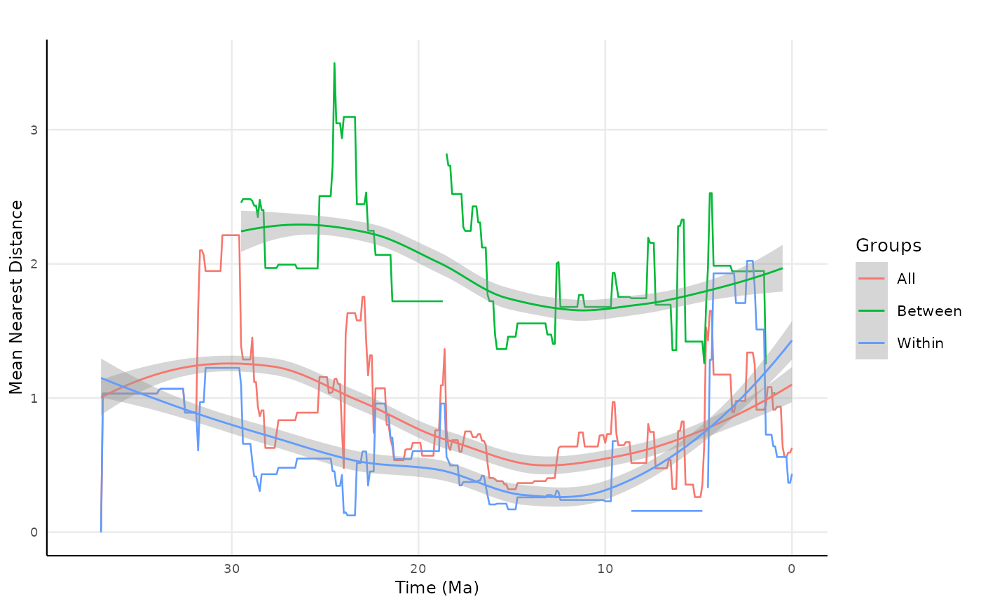
Reach criteria
Reach criteria for coexistence
res_clade_reach_coexistence <-
  clade_reach_coexistence(df.TS.TE = df_longevities_canidae,
                          df.occ = df_occurrence_canidae,
                          time.slice = 0.1,
                          round.digits = 5,
                          species = "species",
                          TS = "TS",
                          TE = "TE",
                          lat = "lat",
                          lon = "lng",
                          Max.age = "max_T",
                          Min.age = "min_T",
                          crs = 4326)
Reach criteria for mean trait distance metrics
res_clade_reach_distance <-
  clade_reach_distance(df.TS.TE = df_longevities_canidae,
                       df.occ = df_occurrence_canidae,
                       time.slice = 0.1,
                       dist.trait = dist_body_mass,
                       nearest.taxon = 1,
                       round.digits = 5,
                       species = "species",
                       TS = "TS",
                       TE = "TE",
                       lat = "lat",
                       lon = "lng",
                       Max.age = "max_T",
                       Min.age = "min_T",
                       crs = 4326)

res_clade_reach_distance_between <-
  clade_reach_distance(df.TS.TE = df_longevities_canidae_trait,
                       df.occ = df_occurrence_canidae,
                       time.slice = 0.1,
                       group = "diet_cat",
                       group.focal.compare = c("meso", "hyper"),
                       type.comparison = "between",
                       dist.trait = dist_body_mass,
                       nearest.taxon = 1,
                       round.digits = 5,
                       species = "species",
                       TS = "TS",
                       TE = "TE",
                       lat = "lat",
                       lon = "lng",
                       Max.age = "max_T",
                       Min.age = "min_T",
                       crs = 4326)

res_clade_reach_distance_within <-
  clade_reach_distance(df.TS.TE = df_longevities_canidae_trait,
                       df.occ = df_occurrence_canidae,
                       time.slice = 0.1,
                       group = "diet_cat",
                       group.focal.compare = c("meso", "hyper"),
                       type.comparison = "within",
                       dist.trait = dist_body_mass,
                       nearest.taxon = 1,
                       round.digits = 5,
                       species = "species",
                       TS = "TS",
                       TE = "TE",
                       lat = "lat",
                       lon = "lng",
                       Max.age = "max_T",
                       Min.age = "min_T",
                       crs = 4326)
Joining the results and plotting
all_mnd_clade_reach <- rbind(res_clade_reach_distance, res_clade_reach_distance_between, res_clade_reach_distance_within)
all_mnd_clade_reach2 <-
  data.frame(all_mnd_clade_reach,
             group_res = rep(c("All", "Between", "Within"),
                             each = nrow(res_clade_reach_distance))
  )
Plotting
all_mnd_clade_reach2 |>
  ggplot(aes(x = as.numeric(time.slice), y = mean.distance, group = group_res, color = group_res)) +
  geom_line(aes(x = as.numeric(time.slice), y = mean.distance)) +
  geom_smooth(se = TRUE, method = "loess", size = 0.5) +
  labs(title = "",
       x = "Time (Ma)",
       y = "Mean Nearest Distance",
       color = "Groups") +
  scale_x_continuous(breaks = seq(max(as.numeric(all_mnd_clade_reach2$time.slice)), 0, by = -10)) +
  scale_x_reverse() +
  theme_minimal(base_size = 10) +
  theme(
    axis.line = element_line(color = "black", linewidth = 0.4),
    axis.title = element_text(size = 9),
    axis.text  = element_text(size = 7),
    axis.title.x = element_text(size = 9),
    axis.title.y = element_text(size = 9),
    panel.grid.minor = element_blank()
  )
#> Scale for x is already present.
#> Adding another scale for x, which will replace the existing scale.
#> `geom_smooth()` using formula = 'y ~ x'
#> Warning: Removed 87 rows containing non-finite outside the scale range
#> (`stat_smooth()`).
#> Warning: Removed 87 rows containing missing values or values outside the scale range
#> (`geom_line()`).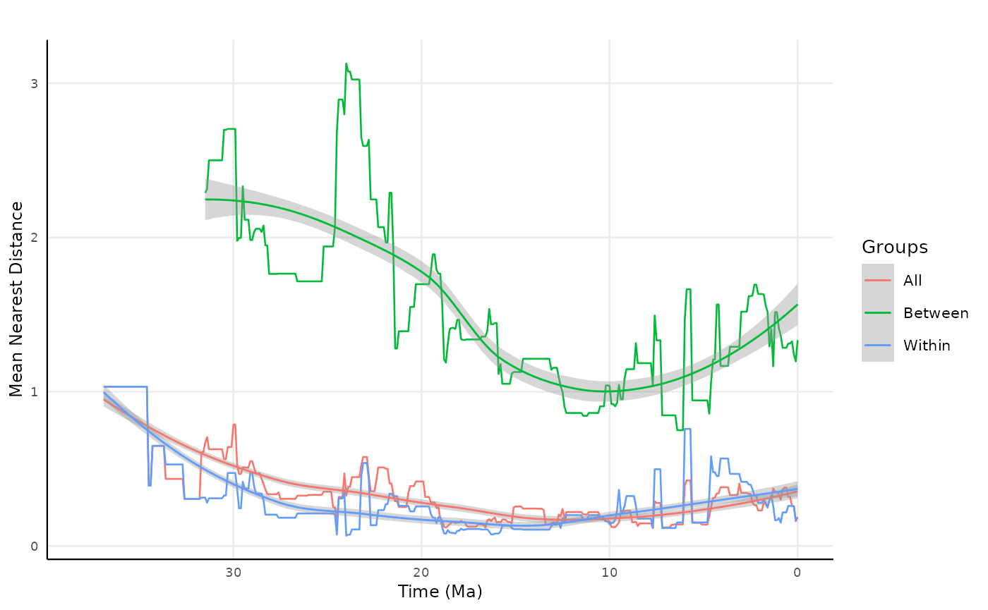
Interspecific Competition at Individual Species Level
In individual species analyses the focus is on the “perception” of each individual species with other co-occurring species. There are two main components in this module. The first computes the number of species in which a given species co-occur. The other is the mean distance between a focal individual and its co-occurring species.
As the other modules there are four spatial levels in which we compute the metrics. The regional level, that calculates the number of co-occurrence by each focal species and all other species with occurrence data in the specified time-slice. The site level, that compute the taxonomic and trait metrics considering as co-existing species only those that present occurrence in the same site (usually defined accordingly to the PBDB definition of a site, or another definition provided by the user). The reach level, that considers a proxy of species dispersal capacity to infer the species that potentially co-occurr. Finally, the assemblage level, that considers as species co-occurring only those with an occurrence record in the same assemblage, this last being defined as a grid of customized size.
Regional scale
res_indiv_species_coex <-
  IndivSpec_regional_coex(df.TS.TE = df_longevities_canidae,
                             time.slice = 0.1,
                             round.digits = 1,
                             species = "species",
                             TS = "TS",
                             TE = "TE")
We can plot the time series for each species
res_indiv_species_coex |>
  filter(
    species %in% c(
      "Aelurodon_ferox",
      "Psalidocyon_marianae",
      "Aelurodon_taxoides",
      "Phlaocyon_marslandensis"
    )
  ) |>
  ggplot(
    aes(
      x = time.slice,
      y = n.coexistence,
      color = species,
      group = species
    )
  ) +
  geom_smooth(
    se = TRUE,
    method = "loess",
    linewidth = 0.8
  ) +
  geom_line(
    linewidth = 0.5
  ) +
  facet_wrap(~ species, nrow = 2) +
  labs(
    x = "Time",
    y = "Number of coexistences by species"
  ) +
  scale_x_reverse(
    breaks = seq(
      from = 0,
      to   = max(res_indiv_species_coex$time.slice, na.rm = TRUE),
      by   = 10
    )
  ) +
  coord_cartesian(clip = "off") +
  theme_minimal(base_size = 10) +
    theme(
    legend.position = "none",
    axis.line.x.bottom = element_line(color = "black", linewidth = 0.4),
    axis.ticks.x       = element_line(color = "black", linewidth = 0.4),
    axis.text.x        = element_text(size = 8),
    axis.line.y.left   = element_line(color = "black", linewidth = 0.4),
    panel.grid.minor   = element_blank(),
    plot.margin = margin(t = 5, r = 5, b = 20, l = 5)
  )
#> `geom_smooth()` using formula = 'y ~ x'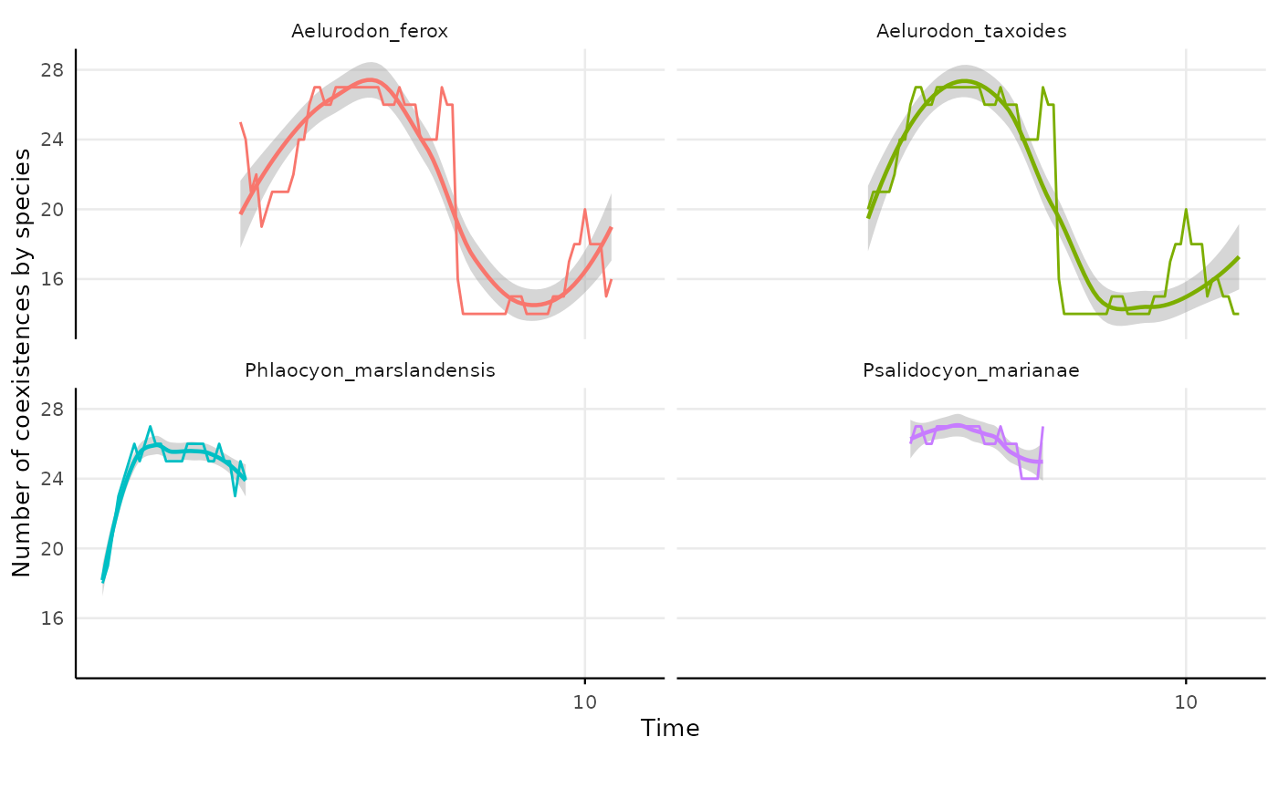
We can also plot individual species mpd for all species coexisting in
regional context. For this we will also use data on body mass for all
species. There are different ways in which mpd can be calculated. We can
calculate it using a single trait or a combination of traits. The later
require a distance trait matrix (passed to dist argument)
containing the pairwise distances among species.
Here we show how to calculate mpd using a single trait, in this case body mass.
res_indiv_regional_species_mpd <-
  IndivSpec_regional_distance(df.TS.TE = df_longevities_canidae,
                              time.slice = 0.1,
                              dist.trait = dist_body_mass,
                              round.digits = 1,
                              species = "species",
                              TS = "TS",
                              TE = "TE",
                              nearest.taxon = "all")
Plotting the results for individual species mpd
res_indiv_regional_species_mpd |>
  filter(
    species %in% c(
      "Aelurodon_ferox",
      "Psalidocyon_marianae",
      "Aelurodon_taxoides",
      "Phlaocyon_marslandensis"
    )
  ) |>
  ggplot(
    aes(
      x = time.slice,
      y = mean_dist_to_cooccur,
      color = species,
      group = species
    )
  ) +
  geom_smooth(
    se = TRUE,
    method = "loess",
    linewidth = 0.8
  ) +
  geom_line(
    linewidth = 0.5
  ) +
  facet_wrap(~ species, nrow = 2) +
  labs(
    x = "Time (Ma)",
    y = "Mean pairwise distance"
  ) +
  scale_x_reverse(
    breaks = seq(
      from = 0,
      to   = max(res_indiv_regional_species_mpd$time.slice, na.rm = TRUE),
      by   = 10
    )
  ) +
  coord_cartesian(clip = "off") +
  theme_minimal(base_size = 10) +
    theme(
    legend.position = "none",
    axis.line.x.bottom = element_line(color = "black", linewidth = 0.4),
    axis.ticks.x       = element_line(color = "black", linewidth = 0.4),
    axis.text.x        = element_text(size = 8),
    axis.line.y.left   = element_line(color = "black", linewidth = 0.4),
    panel.grid.minor   = element_blank(),
    plot.margin = margin(t = 5, r = 5, b = 20, l = 5)
  )
#> `geom_smooth()` using formula = 'y ~ x'
#> Warning: Removed 1328 rows containing non-finite outside the scale range
#> (`stat_smooth()`).
#> Warning: Removed 1328 rows containing missing values or values outside the scale range
#> (`geom_line()`).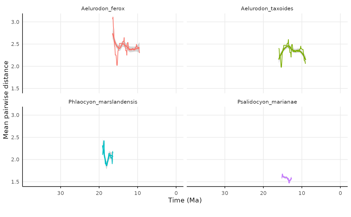
In order to calculate the mpd for multiple traits the user must
inform an object of class dist containing all pairwise distances among
species. The function can handle distances in different ways. It can use
all pairwise distances to obtain the mpd, or the user can inform
throught the argument nearest.taxon the number of nearest
species that will be used to calculate the mpd. The default is
all which is the same as calculating the mpd considering
all species co-occurring in a time slice.
res_indiv_regional_species_mnd <-
  IndivSpec_regional_distance(df.TS.TE = df_longevities_canidae,
                            time.slice = 0.1,
                            dist.trait = dist_body_mass,
                            nearest.taxon = 1,
                            round.digits = 1,
                            species = "species",
                            TS = "TS",
                            TE = "TE")
Site scale
Here we will perform the same calculations but using site criteria for individual species coexistence
res_indiv_species_site_coex <-
  IndivSpec_site_coexistence(df.TS.TE = df_longevities_canidae,
                             df.occ = df_occurrence_canidae,
                             time.slice = 0.1,
                             round.digits = 5,
                             species = "species",
                             TS = "TS",
                             TE = "TE",
                             Max.age = "max_T",
                             Min.age = "min_T",
                             site = "site.char")
plotting species coexistence considering site coexistence
res_indiv_species_site_coex |>
  filter(
    species %in% c(
      "Aelurodon_ferox",
      "Psalidocyon_marianae",
      "Aelurodon_taxoides",
      "Phlaocyon_marslandensis"
    )
  ) |>
  ggplot(
    aes(
      x = time.slice,
      y = n.coexistence,
      color = species,
      group = species
    )
  ) +
  geom_smooth(
    se = TRUE,
    method = "loess",
    linewidth = 0.8
  ) +
  geom_line(
    linewidth = 0.5
  ) +
  facet_wrap(~ species, nrow = 2) +
  labs(
    x = "Time",
    y = "Number of coexistences by species"
  ) +
  scale_x_reverse(
    breaks = seq(
      from = 0,
      to   = max(res_indiv_species_coex$time.slice, na.rm = TRUE),
      by   = 10
    )
  ) +
  coord_cartesian(clip = "off") +
  theme_minimal(base_size = 10) +
    theme(
    legend.position = "none",
    axis.line.x.bottom = element_line(color = "black", linewidth = 0.4),
    axis.ticks.x       = element_line(color = "black", linewidth = 0.4),
    axis.text.x        = element_text(size = 8),
    axis.line.y.left   = element_line(color = "black", linewidth = 0.4),
    panel.grid.minor   = element_blank(),
    plot.margin = margin(t = 5, r = 5, b = 20, l = 5)
  )
#> `geom_smooth()` using formula = 'y ~ x'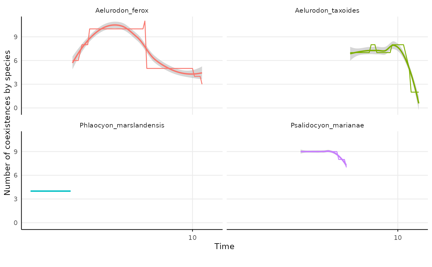
We can calculate mean pairwise distances of individual species coexistence metrics based on site co-occurrence
indiv_species_site_mpd <-
  IndivSpec_site_distance(df.TS.TE = df_longevities_canidae,
                     df.occ = df_occurrence_canidae,
                     time.slice = 0.1,
                     dist.trait = dist_body_mass,
                     nearest.taxon = "all",
                     round.digits = 1,
                     species = "species",
                     TS = "TS",
                     TE = "TE",
                     Max.age = "max_T",
                     Min.age = "min_T",
                     site = "site.char")
Reach criteria
We will calculate individual mean coexistence using reach criteria
res_indiv_species_reach_coex <-
  IndivSpecies_reach_coexistence(df.TS.TE = df_longevities_canidae,
                                 df.occ = df_occurrence_canidae,
                                 time.slice = 0.1,
                                 round.digits = 1,
                                 species = "species",
                                 TS = "TS",
                                 TE = "TE",
                                 Max.age = "max_T",
                                 Min.age = "min_T",
                                 lat = "lat",
                                 lon = "lng")
plotting individual species coexistence with reach criteria
res_indiv_species_reach_coex |>
  filter(
    species %in% c(
      "Aelurodon_ferox",
      "Psalidocyon_marianae",
      "Aelurodon_taxoides",
      "Phlaocyon_marslandensis"
    )
  ) |>
  ggplot(
    aes(
      x = time.slice,
      y = n.coexistence,
      color = species,
      group = species
    )
  ) +
  geom_smooth(
    se = TRUE,
    method = "loess",
    linewidth = 0.8
  ) +
  geom_line(
    linewidth = 0.5
  ) +
  facet_wrap(~ species, nrow = 2) +
  labs(
    x = "Time",
    y = "Number of coexistences by species"
  ) +
  scale_x_reverse(
    breaks = seq(
      from = 0,
      to   = max(res_indiv_species_reach_coex$time.slice, na.rm = TRUE),
      by   = 3
    )
  ) +
  coord_cartesian(clip = "off") +
  theme_minimal(base_size = 10) +
    theme(
    legend.position = "none",
    axis.line.x.bottom = element_line(color = "black", linewidth = 0.4),
    axis.ticks.x       = element_line(color = "black", linewidth = 0.4),
    axis.text.x        = element_text(size = 8),
    axis.line.y.left   = element_line(color = "black", linewidth = 0.4),
    panel.grid.minor   = element_blank(),
    plot.margin = margin(t = 5, r = 5, b = 20, l = 5)
  )
#> `geom_smooth()` using formula = 'y ~ x'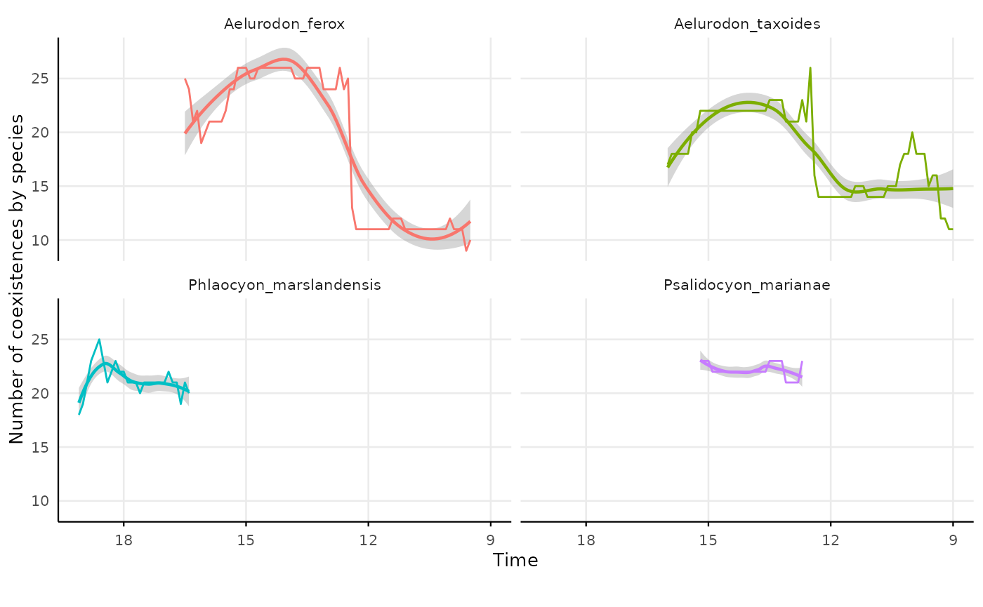
Individual reach coexistence mpd and mnd
res_indiv_species_reach_distance <-
IndivSpec_reach_distance(df.TS.TE = df_longevities_canidae,
dist.trait = dist_body_mass,
nearest.taxon = "all",
crs = 4326,
df.occ = df_occurrence_canidae,
time.slice = 0.1,
round.digits = 1,
species = "species",
TS = "TS",
TE = "TE",
Max.age = "max_T",
Min.age = "min_T",
lat = "lat",
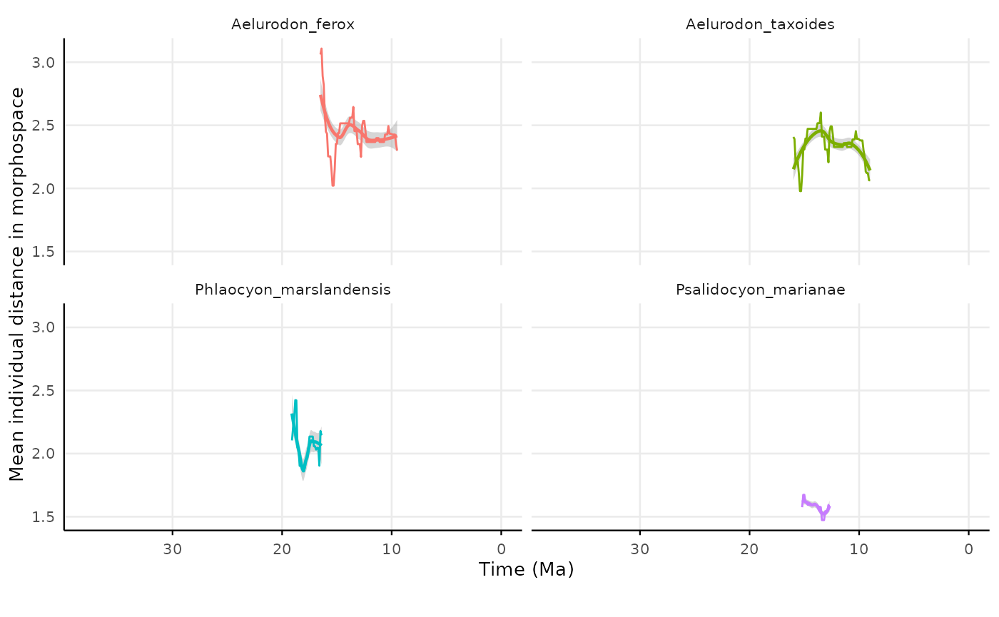
lon = "lng")Plotting the result
res_indiv_species_reach_distance |>
  filter(
    species %in% c(
      "Aelurodon_ferox",
      "Psalidocyon_marianae",
      "Aelurodon_taxoides",
      "Phlaocyon_marslandensis"
    )
  ) |>
  ggplot(
    aes(
      x = time.slice,
      y = mean_dist_to_cooccur,
      color = species,
      group = species
    )
  ) +
  geom_smooth(
    se = TRUE,
    method = "loess",
    linewidth = 0.8
  ) +
  geom_line(
    linewidth = 0.5
  ) +
  facet_wrap(~ species, nrow = 2) +
  labs(
    x = "Time (Ma)",
    y = "Mean individual distance in morphospace"
  ) +
  scale_x_reverse(
    breaks = seq(
      from = 0,
      to   = max(res_indiv_species_reach_distance$time.slice, na.rm = TRUE),
      by   = 10
    )
  ) +
  coord_cartesian(clip = "off") +
  theme_minimal(base_size = 10) +
    theme(
    legend.position = "none",
    axis.line.x.bottom = element_line(color = "black", linewidth = 0.4),
    axis.ticks.x       = element_line(color = "black", linewidth = 0.4),
    axis.text.x        = element_text(size = 8),
    axis.line.y.left   = element_line(color = "black", linewidth = 0.4),
    panel.grid.minor   = element_blank(),
    plot.margin = margin(t = 5, r = 5, b = 20, l = 5)
  )
#> `geom_smooth()` using formula = 'y ~ x'
#> Warning: Removed 1328 rows containing non-finite outside the scale range
#> (`stat_smooth()`).
#> Warning: Removed 1328 rows containing missing values or values outside the scale range
#> (`geom_line()`).